In comparison, to the detection time response of thermal circuit breakers, we can classify the detection time response of magnetic circuit breakers as “fast”.  In many cases, magnetic breakers are in fact “too fast”, and are subject to nuisance trips due to transient inrush currents.  Whereas thermal breakers can “ride through” transient inrush currents by means of their relatively long thermal time constants, magnetic breakers tend to respond to the instantaneous magnitudes of inrush currents due to their relatively low trip energy requirements once the threshold current has been exceeded.

Over the years magnetic circuit breaker designers have developed several schemes to delay the detection response to transient inrush currents.  In essence, the goal is to mimic the dual element “slow blow” fuse structure.  The ideal “dual element” magnetic breaker would have two detection mechanisms in series:  one slow, low threshold current mechanism to ride through inrush currents; and one fast, high threshold current mechanism to quickly respond to true, high level fault currents.  The detection time current response characteristic would look much like the dual-element fuse characteristic shown in Figure 3.9.

A true, almost ideal dual-element characteristic can be achieved in a magnetic circuit breaker through use of an inertial core-delay tube.  This clever device is shown in Figure 4.13a.  The drive coil core is a hollow tube which contains a moveable, but spring restrained core ferromagnetic slug.  At low coil currents the slug is spring restrained in a recessed position, x = 0.

At coil currents above a certain operating current threshold, I_th1, the attractive magnetic force (solenoid effect) of the coil is enough to overcome the spring force and to initiate movement of the slug.  The slug moves toward the coil center and begins to fill the hollow coil core with ferromagnetic material.  As the coil core fills with magnetic material the core section reluctance falls to lower values, enabling the total magnetic flux produced by the coil to increase.  When the core slug reaches a certain point in the core section, dependent on the level of drive coil current, the core reluctance is decreased to a value low enough that the magnitude of the armature gap flux is sufficient to cause the armature to breakaway from its stopped position.  The breaker then trips as described previously.

The dynamics of the slug movement can be further slowed by the addition of a viscous fluid within the hollow core section.

If the initial core current is high enough – above a second threshold level I_th2 – the gap flux will be strong enough to trip the armature without the need of flux enhancement by slug movement through the core section.  The dynamics of this high-level trip are then the fast dynamics of a pure, simple magnetic breaker, unaffected by the flow dynamics of the core slug mechanism.

In terms of a magnetic equivalent circuit, the moveable-core dual element magnetic circuit breaker can be described as shown in Figure 4.13b.  The core path reluctance R_c is now a function of the slug displacement from its restrained x = 0 position.  It is a maximum when the slug is at x = 0, and a minimum when the slug has advanced to its core-filled position at x = x_max.

The equation of motion for the slug is given by

where M_s is the mass of the core slug, F_m is the force of the magnetic attraction on the slug, D is the coefficient of friction due to the addition of a viscous fluid environment, ξ is the spring constant of the slug restraint spring, and x_o is an equivalent displacement representing the initial restraining force of the spring.  The force of magnetic attraction F_m will be proportional to the core flux ф squared (just as the armature attractive torque T_m is proportional to the gap flux ф_g squared).  A complete solution to the dynamics of the total device would then require a simultaneous solution of Equations 4.1 and 4.18, and the magnetic circuit of Figure 4.13b.

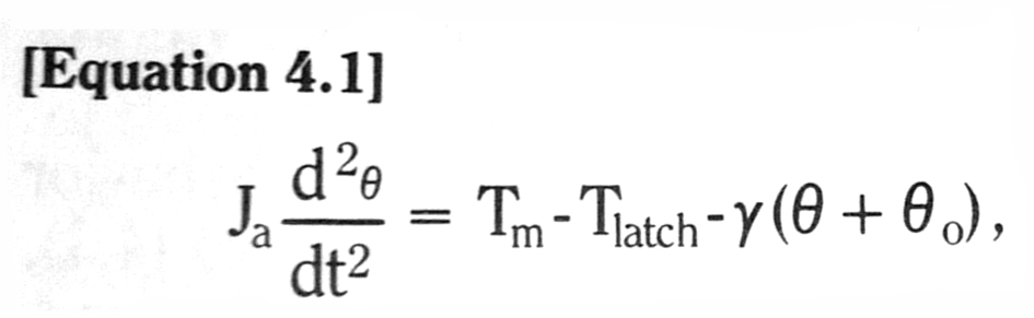
We will not attempt to solve this system of equations here.  We will only note that the “slow” behavior of the complete system is determined by the slug movement Equation 4.18; the “fast” behavior of the system is determined by the armature movement of Equation 4.1; and coupling between the two is determined by the magnetic circuit, Figure 4.13b.  The resultant combined detection time-device current characteristics are sketched in Figure 4.13c.

Other methods of desensitizing the response of magnetic breakers to inrush currents include the tailoring of the core flux reluctance path as a function of the core slug position and the addition of an inertial device, similar to a flywheel, to the armature structure.

Flux can be “bled-off” from the core-gap-armature path through use of flux shunts (sometimes referred to as flux busters) or through the use of an elongated core path which is not covered by the drive coil.  In either situation a major portion of the core flux produced by the drive coil tends not to flow  through the core-armature gap until a movable internal core slug (similar to the one in Figure 4.13a) has reached its fully advanced position.  Rather, this flux “bleeds” into leakage paths, producing no useful armature torque.  However, when the core slug is at its most advanced position these leakage paths are effectively “shorted” and the major portion of the core flux crosses the core armature gap.  Magnetic breakers with these tailored core flux paths have an enhanced, true, dual-element response characteristic.

Extra inertial mass when added to the armature mechanism increases the total effective armature moment of inertia, or equivalently, the total effective armature characteristic time.  This addition does not change the sensitivity of the detection mechanism; it only slows its response.  It slows it, however, across the board.  It does not create the desired dual-element response; rather it simply burdens the armature with additional inertia, enabling it to ride through the transient inrush currents by means of sheer sluggishness.

The production of magnetic flux is instantaneously proportional to the coil current i.  Strictly speaking, this is only true for magnetic circuits which do not contain any electrically conductive magnetic flux paths.  When the level of magnetic flux changes (i.e. is raised or lowered) in a path/medium which can also conduct electric current, such as iron, there will arise, by Faraday’s Law, circulating eddy currents.

(Faraday’s Law states that the voltage induced in any closed path in space is proportional to the time rate of change of the net magnetic flux which flows through the closed path cross-sectional area.  If the closed path is in an electrically conducting medium, there will then be a circulating current around that closed path proportional to the generated voltage and the electrical conductivity of the medium).

These eddy currents will, in turn, produce reaction magnetic flux which will tend to cancel out a portion of, or all of, the original excitation flux.  The direction of eddy current flow can be deduced by the “ right hand rule” and by the requirement that the reaction magnetic flux produced by the eddy currents must flow in the opposite direction to the flow of excitation flux.  Eddy current production in a simple cylindrical path in iron is illustrated in Figure 4.11.

As a result of eddy currents, flux cannot be instantaneously produced in conducting mediums.  There will always be a time “lag” between the flux flow and the exciting mmf.  A simple magnetic equivalent circuit representation of this time-delay effect can be made by including “inductive” elements in series with reluctance elements which represent electrically conductive paths.  For example, the structure shown in Figure 4.4 has two magnetic paths which are made up of ferromagnetic material: the core path and the armature path.

We include eddy current effects in these two paths by placing inductive elements in series with the reluctive elements which represent these paths.  This modified circuit is shown in Figure 4.12.

The value of the inductive element for each magnetic path in a conducting medium is a function of the cross-sectional geometry of the path, the electrical conductivity of the material, and the effective length of the path.  In the simple cylindrical structure of Figure 4.11, it can be easily shown that the equivalent eddy current inductance L_e is given by

where L is the axial length of the conductor and ϱ_r is the electrical resistivity of the material.  The magnetic reluctance of this path is

where µ_m is the magnetic permeability of the material , A is the cross-sectional area = πr², and r is the cylinder radius.  The magnetic time constant τ_e of this cylindrical path is then

As typical values, let the material be a 1.5mm radius rod of magnetic iron with µ_m=˜ 2000µ_o and ϱ_r = 10^-5Ω-cm.  Thus,

If such a rod is used as a magnetic core in a magnetic circuit breaker, and if we wish to accurately predict the breaker time response over time intervals of this magnitude, we must then necessarily include eddy current effects in our calculations.  We can no longer use the simple results for the gap flux calculated from the static circuit of Figure 4.4.  Rather, we must use the dynamic circuit of Figure 4.12.  Results such as those given in Figures 4.9 and 4.10, calculated using static equivalent magnetic circuits, are optimistic at predicted operating time intervals equal to or less than the eddy current time constants of the structure elements.

For a rectangular cross-section magnetic path with side length ratio k, the equivalent eddy current inductance can be shown to be equal to

The path lengths of eddy currents in a rectangular cross-section magnetic conductor are longer than those in circular cross-section magnetic conductor.  Thus, for equal electrical conductivities, the effective eddy current inductance in a rectangular conductor is lower.

To mitigate eddy current effects in magnetic materials, we see from Equations 4.16 and 4.17, that we should construct magnetic cores with

1)     Magnetic irons (steels) with high resistivity values, (i.e. silicon steels). And

2)     Very thin sheets (i.e. laminations) of magnetic steels stacked in the thin direction, and oriented such that the thin direction is perpendicular to the flow of magnetic flux.

The cost of such construction is only justified for devices which must operate at very high speeds (i.e. operating periods of the order of milliseconds).

We can recast the equation of motion.

Equation 4.1, in dimensionless form by dividing through by the breakaway torque T_B.  We obtain

The quantity J_aθ_g/T_B has units of (time)², so we define a characteristic time t_a for a magnetic breaker as

This “time” is seen to be a function of the inertia of the armature, the spring constant of the armature restraining spring, the amount of pre-load we place on the restraining spring, and the angular width of the armature air gap.  Each different magnetic breaker will have its own particular value of t_a.  But in terms of t_a, all magnetic breakers of similar design will have the same dynamic behavior.

If we assume the idealized case of no latch mechanism load torque (i.e. T_latch = 0), we will not need to consider impact effects when the armature slams into the latch mechanism.  This case will also be the minimum time response, or fastest possible response, for a magnetic structure.  The normalized equation of motion can then be written as

We can easily solve this differential equation numerically for any given set of values for the frame reluctance fraction m, normalized coil current i/I_th, and gap angle – spring pre-load angle ratio θ_g/θ_o.  Example solutions for m = 0.1, θ_g/θ_o  = 1.0, and different values of step input i/I_th are given in Figure 4.9.

The latch mechanism trips the contact separation mechanism when the armature angle reaches the latch threshold value θ_th.  The time required to trip the contact separation mechanism, measured from the overcurrent inception, is the detection time of the breaker t_d.  We plot the detection time response for the example solutions given in Figure 4.9 as a function of input normalized overload current in Figure 4.10.

In this case we have assumed that the threshold armature angle is 80% of the armature gap angle.  As can be seen, the normalized detection time is a monotonically decreasing function of the normalized input current.

In the case of no armature saturation, at high values of input current (in the example of Figure 4.10 for i>5I_th), the detection time becomes linearly dependent on the ratio I_th/i.  This linear behavior at high input currents can be deduced directly from the normalized equation of motion.  At high input currents the armature angular acceleration is approximately proportional to (i/I_th)² only.  Thus a simple double integration gives

From which we see that

for a given threshold angle θ_th.

If armature saturation occurs, the time response of the armature will be slowed slightly.  The detection times for a saturated case would be slightly higher than non-saturated values, such as those given by the solid line in Figure 4.10.Saturated values would tend to level off at a minimum detection time since the drive torque would also saturate at a maximum value, given by (4.9) using the saturated gap flux value.  A typical saturation case is shown by the dashed line response in Figure 4.10.

Magnetic circuit breakers have DC threshold currents.  When magnetic devices are operated at their threshold levels, the trip or detection times are also “long” times.  Action on the onset of mechanical movement in a magnetic circuit breaker, however, is more abrupt than in a thermal circuit breaker.

Mechanical movement of the thermal element is evident up to the detection threshold value in a thermal breaker.  In a magnetic breaker, there is the possibility of no mechanical action, (i.e. no movement whatsoever) until the threshold current is exceeded.

From the equation of motion (4.1) we have that there will be a net accelerating torque on the armature at angular position θ = 0 whenever

where we have assumed that the latch mechanism is not engaged until θ>˭θ_latch.  We will term the torque value ƴθ₀, the breakaway torque T_B.  If we now plot the load torque – the restraining spring plus latch mechanism – as a function of armature angular position, we obtain a load torque locus such as that shown in Figure 4.5.

Note that we have approximated the load torque of the latch as a constant average torque, <T_latch>, over the operating range of latch mechanism.  We also show the load torque diminishing (dashed line) after the latch release angle θ_th.  In truth, we care little as to the actual behavior of armature after tripping, and therefore the true locus after this point is of no concern.

From Equations 4.9 and 4.11,

we see that the driving torque of magnetic attraction T_m is given by

The current needed to produce a torque of magnetic attraction equal to the breakaway torque will be termed the threshold current I_th, and is defined by the expression

Equation 4.12, the equation for the magnetic torque, can then finally be written in a compact form as

We can now plot, for a given value of frame reluctance fraction m and various values of constant coil current i, the value of magnetic drive torque T_m as a function of the armature angle θ.  These curves are shown, along with the load torque curve T_L, in Figure 4.6.

The difference between the drive torque T_m and the Load torque T_L at any value of armature angle θ, is the acceleration torque.  Once the threshold current I_th has been exceeded, the net acceleration torque T_m – T_L is seen to increase as the armature approaches its closed position.  This is a positive feedback effect, contributing to the “fast” characteristic behavior of magnetic circuit breakers.

In some magnetic breakers, the positive feedback effect is diminished somewhat by magnetic saturation of the armature iron.  As the armature gets closer to its closed position, the gap reluctance becomes smaller.  Thus, the total reluctance of the armature-gap path also becomes smaller, which for constant coil current, induces higher levels of armature-gap flux.  If this level of flux approaches the saturation level of the armature, the effective armature reluctance R_ca begins to rise, and thus the frame reluctance fraction m begins to rise as well.

The effect of a rising value of m, due to armature saturation for a constant coil current i, is shown in Figure 4.7. 

Here, curves of drive torque T_m at constant coil current i, but varying values of frame reluctance fraction m, are plotted as functions of the armature angle θ.  If armature saturation occurs as θ approaches θ_g, the actual trajectory of T_m would be along a curve, such as the one shown as T_m (sat).  The net accelerating torque over the operating range of θ is thus seen to diminish, if armature saturation is present.

We have defined the threshold current as that coil current which induces a value of magnetic torque of attraction equal to the armature breakaway torque.  There are situations, however, where this definition is inadequate.  For example consider the drive torque – load torque case shown in Figure 4.8.

Here, an impressed coil current is of sufficient magnitude such that

                                              T_m (θ = 0) > T_L (θ = 0)

so the armature would start to move.  But, at an armature angle value θ_A, less than the latch angle θ_th, the drive torque curve crosses over the load torque curve.  This cross over point, point A, is a stable operating point (net accelerating torque for θ<θ_A and net decelerating torque for θ>θ_A), and thus motion will stop at A.  The “trip” threshold drive torque curve for this situation is shown by the dashed line in Figure 4.8.

Situations such as the one shown in Figure 4.8 should be avoided in the design of magnetic circuit breakers.  Breakers designed as in Figure 4.8 will always exhibit a certain value of armature overshoot, beyond angle θ_A, due to the armature inertia.  If this overshoot is large enough, the latch mechanism could be tripped inadvertently.  Rather than depend on the uncertain impact behavior between an overshooting armature and the latch mechanism, the design of a magnetic circuit breaker trip-threshold should be based on the behavior indicated in Figure 4.6.  Namely, no armature movement should occur until the coil current exceeds the threshold value.  We can insure this type of response simply by requiring that the drive torque curve never cross-over the load torque curve at any value of θ, including θ>θ_latch.

The magnetic flux ф_g that flows through the air gap in the structure of Figure 4.2, is a portion of the total flux generated by the current flowing in the coil which surrounds the core material. 

This total flux ф, which flows through the coil enclosed cross sectional area, is produced by the coil current and is proportional to both the magnitude of the coil current i and the total number of turns N of wire that makes up the coil.  The product of N and i is referred to as the magnetomotive force, or mmf, of the coil.  The proportionality factor in the relationship between the total flux produced by the coil current and the coil mmf, has units of flux (measured in webers) per unit mmf (measured in ampere-turns). 

Since the total flux ф is proportional to a force term – the mmf – a simple analogy can be made between a magnetic circuit and an electrical circuit.  In a DC electrical circuit the current i flows due to an electromotive force (emf) E.  Ohm’s Law for an electrical circuit states that

where R is the resistance of the circuit to the flow of current.  A “Magnetic Ohm’s Law” is then

where R is the resistance of the magnetic circuit to the flow of flux.  This resistance to flux flow R has been assigned a special name to differentiate it from resistance to current flow.  We refer to it as the reluctance of the magnetic circuit.

The reluctance of a magnetic circuit will be approximately constant as long as the flux density in any one portion of the circuit is below the saturation flux density for that portion of the circuit.  Ferromagnetic materials become saturated with magnetic flux at density levels of approximately 1-2 Teslas = 1-2 webers/(meter)².  At density levels near this saturation value, the effective reluctance of the material rises rapidly.  At density levels below the saturation value, the reluctance of ferromagnetic elements is far below that of comparable sized elements constructed of non-magnetic materials.

To construct a representation of a simple lumped magnetic circuit for the magnetic circuit breaker structure of Figure 4.2, we must remember that the total flux created by the coil to be made up of two components:  a gap component ф_g which flows through the coil, the core structure, the armature and the gap, and a leakage component ф_ᵜ which flows through the coil, a portion of the core structure and a leakage air path.  Figure 4.4a illustrates the two components flowing in their physical paths.

Figure 4.4b illustrates an electrical equivalent “magnetic circuit” for the device.  Here, the coil mmf is shown as a DC voltage source of magnitude Ni, and the magnetic reluctances of the different flux paths are shown as equivalent resistances.

The reluctance portion of the core which carries both the leakage flux and the gap flux is labeled R_c;  the reluctance of the air path portion of the leakage flux path is labeled R_ᵜ; the reluctance of the core and armature portion of the gap flux path is labeled R_ca;  and the gap reluctance is termed R_g.  The actual values of the reluctances R_c, R_ᵜ, R_ca and R_g are determined by the effective cross sectional areas of the respective flux paths, the effective lengths of the respective flux paths, and the magnetic permeabilities of the respective flux paths.  If the path material is a ferromagnetic material, such as iron, the path reluctance will also be a function of the level of flux density within the path, if the density level is near or above the saturation value.

In general, for any given path, we have for the path reluctance

where L_p is the effective length of the path, A_p is the effective cross sectional area of the path, and µ_p is the magnetic permeability of path medium.  If the path medium is ferromagnetic, at high levels of path flux, ф_p, flow, we have µ_p = µ_p (ф_p).  Since the gap flux and the leakage flux are both air paths, both path permeabilities equal the permeability of free space µ_o – which is a strict constant, and not a function of path flux level.

For the gap we have approximately

where θ_g is the angular opening of the gap measured with the armature at its held position.  If we define

we then have

Now from simple DC circuit analysis of the circuit of Figure 4.4b, we have

or, if we normalize the circuit reluctance as “seen” from the gap, R_ca  + R_ᵜ  R_c /(R_ᵜ + R_c)to the maximum gap reluctance R_gmax, and let this ratio be termed the frame reluctance fraction m, we have

Since the core and armature are constructed with magnetic materials, we have in general,

This last result suggests that the frame reluctance fraction m is a small quantity.  At high levels of core or armature saturation, however, these approximations become less accurate and the value of m will grow.  Some devices are constructed with a “time-engineered” value of R_c.  For the “time-engineered” devices, the core flux path reluctance R_c is high for a portion of their operating time.  Thus the above approximations are also invalid.

It is well known that electromagnets can exert a lifting or attractive force on ferromagnetic materials, such as iron.  The force mechanism is the same mechanism by which permanent magnets attract iron objects.  Simply stated, near the surfaces of a magnetic material (a ferromagnetic material, one which has a low resistance to the flow of magnetic flux), the density of the energy stored in the magnetic field is much higher on the exterior than on the interior of the material.  By the principal of virtual displacement, there will be a mechanical pressure in the direction of the outward normal at the surface of the magnetic material.  Since there will be more magnetic field flux at the surfaces of the material that are closest to a nearby magnet, or electro-magnet, the total net force on the magnetic material body will be an attractive force, towards the magnet or electromagnet.

Consider the electromagnet structure shown in figure 4.1

In it a coil of N turns of wire is wrapped around one leg of a ferromagnetic core structure.  A movable ferromagnetic armature is hinged to another leg of the core structure.  At one end position of swing the armature closes the core structure and completes a closed path of ferromagnetic matter through which magnetic flux can flow.  The armature is held away from the core closing position by a spring mechanism, creating a classic "relay" structure.

Coil current will induce magnetic flux within the core material, the armature material, and in the gap between the armature and the coil leg of the core.  At a sufficient level of coil current the magnetic attractive force on the armature will exceed the retention force of the spring and the armature will move to its core closed position.  If, by its movement, the armature can trip a latch mechanism - releasing a spring driven contact opening mechanism - then based on the level of coil current, we have a trip/no trip decision mechanism (i.e. we have a magnetic circuit breaker).

A simplified armature-latch release mechanism is shown in Figure 4.2.

Observe that the armature's path is composed of two sections, a free-movement (spring constraint only) portion, and a latch release (spring constraint and latch restraint force) portion.  It is similar to the deflection path of the bi-metallic element in a creep type thermal circuit breaker.

 The equation of angular motion of the armature (see Figure 4.3) is given by

where θ is the armature’s angle, measured from its completely restrained position; θ_o is an angle measure of the initial pre-load on the restraining spring; γ is the torsional spring constant of the restraining spring; T_latch is the torque load of the latch release mechanism (T_latch = 0 during the free movement portion of the armature travel); T_m is the torque due to magnetic attraction, and J_a is the effective angular moment of inertia for the entire armature structure.

In equation 4.1 we have neglected all friction effects due to the armature hinge and air movement.  For this structure, the detection time t_d is defined as the time, measured from the overcurrent inception, required for the armature angle θ to advance to the point of latch release.  We will define this latch release angle as θ_th.

Before discussing the dynamic behavior of the armature, that is, solutions to (4.1), we will first examine the nature of the magnetic torque T_m.  Neglecting any magnetic flux paths through the top surface of the armature structure, the total magnetic torque on the armature is given by

where the surface integral is taken over the entire armature bottom surface (the surface on the core side), p_m is the magnetic pressure on the armature bottom surface, and r is the moment arm of the differential force p_m dA.  Since the armature is made of iron, the direction of magnetic flux flow through its exterior surface will be almost perfectly normal to the surface.  In this case, the magnetic pressure [4.1] is given by

where B_n is the magnitude of the normally directed magnetic flux density vector at the armature surface, and µ_o is the magnetic permeability of free space (µ_o = 4π x 10^-7 henries/meter).  The magnetic permeability of a medium is a measure of the medium’s ability to conduct the flow of magnetic flux.  Magnetic materials have relative permeabilities several thousand times that of free space.  The total net magnetic force F_m on the armature, directed towards the core structure, is given by

And the total magnetic flux ф_g, which flows through the bottom surface of the armature, and therefore, through the gap between the armature and the core, is given by We can now define an effective gap cross-sectional area A_g by equating the two force expressions

Such that

This effective gap cross-sectional area allows us to think of the armature as a free body, with a uniform magnetic pressure F_m/A_g, acting on a portion (A_g) of its lower surface.  We can even define an effective moment arm r_q for a point force F_m by equating

So that

If the distribution of normal magnetic flux over the bottom surface of the armature does not change as the armature position or the driving coil current changes, the effective cross-sectional area of the gap A_g, and the effective armature moment arm r_q, will both be constant (See Equations 4.6 and 4.8).The total magnetic torque on the armature is now simply given by

Equation 4.9 indicates that in order to increase the magnetic torque for any given armature structure, we need only increase the total gap flux.  And, for a given input current, we need only to control the time development of the total gap flux, if we wish to control the time response of a magnetic breaker detection mechanism.

In a bi-metal thermal circuit breaker, the elements expand in longitudinal directions, but the major or useful mechanical movement is in a lateral direction to the elements.

 Consider the two blade elements, 1 and 2 shown in Figure 3.15a.

A blade is a body with an elongated, rectangular cross-section, and with overall length L much greater than either the width b or thickness h.  Both blades have equal length L_o at a reference temperature T_o.  But, at temperature rise ΔT = T-T_o, blade 2 is longer than blade 1, L₂>L₁, because the difference in the two coefficients of thermal expansion, α_t2>α_t1.

If we now bond the two blades together while at the reference temperature, to form a single blade of thickness h = h₁ + h₂, we produce a bi-metal blade element see Figure 3.15b).  Now, at temperature rise ΔT, blade 2 will try to expand to length L₂, but will be “held back” by its bond to blade 1.  Blade 1 wants to expand only to length L₁, but it is “pulled” to a length greater than L₁ by its bond to blade 2.  Thus, blade 2 is subjected to an overall longitudinal compressive force P₂, while blade 1 is subjected to an overall tensile force P₁.  Since there is no movement of the total free body when the elevated temperature is held constant, these two forces must be equal and opposite along the length of the total composite blade.  The curvature seen in Figure 3.15b, will be concave (an inside curve) on the blade 1 side and convex (an outside curve) on the blade 2 side.

The formal definition of concave curvature is

We might (correctly) suspect that for small values the concave curvature of the composite blade would be proportional both to the temperature rise ΔT of the blade and to the difference in coefficients of thermal expansion of the two blade materials.  That is,

and K is a proportionality constant which would be a function of the elasticity of each blade material and the thickness of each blade.  Neglecting small end effects, the radius of curvature should be a constant along the length of the composite blade, so that K should not be a function of the original length L_o.  K should also not be a function of the width b, if L_o is several times larger than b, since the major bending will only be along the longitudinal axis.

The original derivation of the proportionality constant K is credited to Villarceau, who published his work in Paris in 1863.  The standard English language derivation of K is the classic 1925 paper of Steven Timoshenko, “Analysis of Bi-Metal Thermostats.”  In this paper Timoshenko not only derived the bending constant K, he also presented for the first time, the theory of “snap action” thermostat behavior. 

Timoshenko has shown that for an amazingly large range in elastic material constants, and for an amazingly large range in blade thicknesses, the bending constant K can be approximated as

Figure 3.16 illustrates that for a free blade, we can them solve for the maximum mid-blade deflection ό as follows:

The curved blade arc angle φ is given by

where ΔL is the composite blade terminal expansion.  But for small deflections, L_o/r is already small so that the term ΔL/r is of second order and can be neglected, thus, φ =~L_o/r.

The cosine of φ/2, by the construction shown in Figure 3.16, is

which for small φ can be approximated by

For a blade built into a fixed wall – a cantilever beam – we see from Figure 3.17 that the blade end deflection is exactly the same as the mid-blade deflection of a free blade of initial length 2L_o.  Thus, for a cantilever blade of initial length L_o, we have for the blade end deflection

Note that for equal lengths, the maximum deflection of a cantilever blade is four times that of the free blade.  We can now combine (3.14) and (3.15) with deflection Equations 3.16 and 3.17 to obtain:

Normally a creep bi-metal blade must not simply deflect - it must also exert a force on a latch release mechanism during a portion of, or during all of, its deflection trajectory. 

From the elementary theory of uniform beam deflections, we have for the configurations of Figure 3.18 that the deflections for a concentrated mechanical force P_m are

where E is the effective Young’s modulus of elasticity for the composite blade.  It follows that a bi-metal blade will exert a concentrated force P_m if it is constrained such that if it was free it would deflect by an amount ό_m.  Thus, to calculate the temperature rise ΔT needed to deflect a blade by an actual distance ό, and to exert force P_m, we use the equivalent deflection ό_eq,

This equivalent deflection would be used in place of the actual deflection ό in Equations 3.18 and 3.19.

Let us subtract from any free deflection ό_f that a blade would travel before exerting any mechanical force on a latch mechanism.  This free travel deflection would be subtracted from the total actual deflection ό, and the total equivalent deflection ό_eq.  We then have

where we can define

an equivalent free deflection while exerting a mechanical force on the latch mechanism and

an actual deflection while exerting a mechanical force on the latch mechanism.  So that

If we assume that the average amount of work, W_m, expended in tripping the latch mechanism is equal to a constant average mechanical force P_m, times the action distance ό’, using (3.18) through (3.21) for both free and cantilever blades, we have

where we differentiate between free and cantilever blades by the factor β, where

and ΔT’ is the temperature rise needed to deflect the blade a total equivalent distance of ό’_eq.  We can simplify (3.24) and place it in the form

where the constant W_k = 9/64 β⁴E (Δα_t)², m = ό_m/ό’_eq and L_obh is the total volume of the blade material.  Thus, for a given latch mechanism which requires energy W_m to trip, and for a given desired operating temperature rise ΔT’, we can determine the most economical blade design - (i.e. the minimum volume design) if we minimize the expression for the total blade volume

with respect to the normalized suppressed mechanical travel m = ό_m/ό’_eq.  By taking the derivative of (3.25) with respect to m, and setting it to equal zero, we find that the optimum design is one with

That is, the suppressed deflection should be equal to the actual deflection when the blade is in the process of exerting a mechanical force.  Any other choice of deflection ratios will result in an increase in the required volume of bi-metallic material, and thus an increase in material cost.  Note that the amount of free travel that the blade undergoes before it begins any mechanical work has no effect on the optimum choice of suppressed blade deflection.  This free travel only influences the total amount of temperature rise that is needed to complete the total equivalent deflection.

As a practical example of a minimum volume design, consider the use of Chace No.2400 bi-metal material in a cantilever blade latch release mechanism.

In our notation, the manufacturer supplied data for this representative material is given in Table 3.1.  Assume that the blade must, after some length of free deflection, push against a latch mechanism with an average force of one once.  And to trip the mechanism the blade must travel 0.05 in. while applying this force.  The work required to trip the latch is then

Further assume that we wish this work to be accomplished by a deflection due to temperature rise ΔT’ = 50^oF.  From Equation 3.25 with W_k = 5.74 x 10^-3 1bf/(in^2oF), the minimum volume of material that is capable of performing this work (i.e. the m = ½ design), is given by

A commonly available thickness value for bi-metal material is 0.008 inches.  If we choose this value for h, and assume an active blade length of ¾ inch, we see that we need a blade width of,

Note that this minimum volume design satisfies our original assumptions of a “blade” device, one with a length several times greater than width or thickness.

The time it takes for a creep bi-metal element to trip a latch release mechanism is the time it takes to heat the element to the required total temperature rise ΔT = ΔT_f,+ΔT’, where ΔT_f, is the temperature rise during any free deflection of the element before it begins any latch release work.  We can safely neglect any inertial effects due to the bi-metal element itself.  The stiffness of bi-metal material insures that the transient or natural mechanical response of the element is completely negligible in comparison to the driven mechanical response for any reasonable level of heat application.  This can be easily seen if one calculates the period of the fundamental frequency of natural vibration of a bi-metal element.  This period is much less than the time needed to raise the temperature of the element to the value dictated by the required total deflection.  Thus the time-current detection period characteristics of a directly heated bi-metal element can be determined exactly like those of a hot-wire element.  That is, we can use Equation 3.9, with suitable values for the constants: threshold current I_th, element resistance temperature sensitivity factor k, and element thermal time constant Ƭ. 

For an indirectly heated bi-metal element, the thermal equivalent circuit is more complicated than the simple two element model.  An indirectly heated element analysis must, at a minimum, involve two thermal time constants – one for the actual heating mechanism and one for the bi-metal element itself.

For a directly heated element we can solve for the time-current response using Equation 3.9 as follows:

1)      1) Choose a desired threshold temperature rise ΔT = ΔT_f + ΔT’.

2)      2) For the particular blade element material, find the resistance temperature factor k from

3)      3) Integrate (3.9) numerically.

As an example, let us solve (3.9) for Chace No. 2400 material.  If we choose a threshold total temperature rise of 200^oF, we have

The actual value of the long time threshold current I_th is best determined experimentally since it depends on the thermal resistance R_t, which is unknown and not easily theoretically determined.  In normalized form, the solution for stepped DC currents for the detection time t_d, the time required to reach T_th, is given in Figure 3.19.

In general, due to the differences in thermal capacity, the thermal time constants for hot wire breakers will be smaller than those of thermal creep-blade breakers.  Thus, the actual detection times, for equal ratios of operating current to threshold current, will be related by

T_d (hot wire)< t_d (creep-blade)

Finally we note that thermal “creep” type breakers must be derated at high ambient temperatures.  However, by special design, such as the addition of a second bi-metal (complimentary) mechanism, thermal breakers can be ambient temperature compensated.  These compensated mechanisms show little variation over their specified operating temperature range.

In a hot wire circuit breaker a wire of length x₀ at reference temperature T₀ will expand by length Δx=x₀a_tΔT for temperature rise ΔT.  This temperature rise, as in a fuse element, can be generated by the I²R loss in the wire itself. 

If a given wire extension Δx_trip trips a latch mechanism, which releases a contact separation mechanism (see Figure 3.13), the needed temperature rise within the wire at the detection threshold is then

We now have a situation exactly analogous to that of the detection mechanism in a fuse.  The exception is that we need only raise the element temperature to the value given by (3.8), not to the melting point.  The thermal circuit analysis Equations 3.1 through 3.4, with suitable notation changes, also apply to the hot wire thermal circuit

We define

A_r = the wire temperature coefficient of resistivity,

R_o = the wire resistance at the reference temperature,

R_t  = the thermal resistance of the wire to the surroundings,

I_th = the steady-state DC current which will raise the temperature by ΔT_th (i.e. the long trip time current),

k  = the wire resistance temperature sensitivity factor = a_rI_th²R_oR_t  and C_t = the wire thermal capacity.

Thus, just as in Equation 3.4 for a fuse, we have for the hot wire temperature rise ΔT, and for any current I (t)

where is the wire thermal time constant

As an example, consider the use of an 80% Nickel – 20% Chromium alloy wire, which has the trade name Nichrome V.  This alloy has the average properties:

Reference resistivity:  ϱ_o = 108 x 10^-6 Ω-cm (20^o)

Coefficient of resistivity:  α_r = 1.1 x 10^-4/⁰C (20-500^o C)

Coefficient of expansion:  α_t = 1.7 x 10^-5/^oC (10-1000^oC)

Specific heat:  C_p = 435 J/kg^oC.

Assume that the relative extension of the wire at the trip threshold Δx_trip/x_o is to be 0.5%.  Thus, by (3.8)

If we choose #30 wire (American wire gauge) we have the following data from the manufacturer:

Wire diameter:  0.010 in

Resistance at reference temp:  R_o = 6.500 Ω/ft(20^oC)

Mass:  2.86 x 10^-4 lbm/ft

Long time heating current for horizontal wire in air:

The wire thermal capacity per foot is then

If we use the free air heating-temperature data at I (RMS) = 1.21 A, we have for the wire resistance  R

Thus

The free air thermal time constant is then

The long time threshold current is

And the wire resistance temperature sensitivity factor k is

We can now, as we did for the equivalent fuse link, solve for the time it takes for the wire to reach its threshold temperature as a function of current.  These solutions are given in Figure 3.14.

Note that for Nichrome V the resistance temperature sensitivity factor is so low that we can, as a fair approximation, neglect the k multiplied term in (3.9) and solve the resulting equation analytically as

The time to reach the threshold temperature rise t_d is then given by

Which, for long (i/I_th)², reduces to

All interruption devices absorb energy from the circuit in which they operate.  Even a simple mechanical switch absorbs energy within its switching arc during the time period the arc is present.  How much energy the switching device can absorb, and still function in additional operations, is a measure of the device’s interrupt rating.  For example, the on/off switch in a laboratory power supply is rated to switch x number of amps at a given level of input line voltage.  Such a switch, however, is not designed to interrupt high levels of overcurrent and could fail (i.e. be destroyed) if it is used to do so.  The switching contacts in a circuit breaker, however, are designed for overcurrent interruption.  And thus, a breaker in series with an on/off switch would have a higher interrupt rating than that of the switch. 

A portion of the energy absorbed during the operation of an overcurrent protection device is used in the overcurrent detection process.  Since detection is a binary trip/no trip decision process, there must exist a threshold portion of the total absorbed energy within the device which will trigger the device’s interruption process.

In a fuse, the threshold is reached when the fuse element melts and begins to vaporize within a portion of its length.  In a thermal circuit breaker, the threshold is reached when a certain level of thermally induced expansion or deflection is attained within the thermal element.  In a magnetic circuit breaker, the threshold is reached when a movable armature has been magnetically attracted to a certain position.

We will term the detection threshold value of energy W_dt.  The time period between the initiation of the circuit overcurrent, and the time at which the absorbed energy within the detection mechanism of the protection device surpasses W_dt, is termed the detection period t_d (see Figure 1.5).  If the overcurrent is initiated at time t=0, we then have

where W_d is the total amount of energy absorbed within the protection device during the detection period.  v_B is the voltage drop across the device terminals, and i_B is the device current.  Note that in all cases                                                                                                                                          W_d > W_dt

 but only slightly, due to inefficiencies within the protection device internal circuitry.  Such inefficiencies include contact resistance losses, wiring resistance losses, conduction heat transfer away from thermal elements, etc.

The interruption period of a protection device begins immediately after the detection energy threshold has been exceeded.  Within this period, metal vaporization evolves into an arc in a fuse, and contacts separate and initiate an arc in a circuit breaker. The total energy absorbed by the device during this period, W_i, is given by where t_c is the total clearing time of the interruption device (see Figure 1.5).  Within the interruption period t_i = t_c-t_d, is the arc time t_a, where t_a ≤ t_i.  The energy absorbed within the arc, W_a, is given by

 where v_a is the voltage drop across the device arc.  In all practical devices, the arc voltage drop dominates the device voltage so that v_a =~ v_B, and the dominant portion of the total energy absorbed during the interruption period is consumed in the arc.  Thus, W_a =~ W_i.

The total clearing energy absorbed, W_c, by the protection device during the total clearing time t_c, is then given by            

It is this total absorbed energy W_c which doubly concerns the protection device designer.  In many cases the designer would like the detection threshold energy W_dt to be small, such that for large overcurrents the detection period can be short and the total W_c small.  But the designer would also like the device to be tough, (i.e. be able to interrupt very large overcurrents, with their associated large W_c’s), and survive.  Within these two conflicting goals lies a compromise design.

Nowhere is this compromise more evident than in the design of a thermal circuit breaker.  It is obvious that the detection of overcurrents by thermal means can be fast.  A high speed semiconductor fuse is, in fact, the fastest electromechanical protection device available.  But a fuse can afford to be fast, since it is designed to self-destruct when it operates.  It is deliberately designed to have a low thermal mass.  Thus, it can reach its operation (melting and vaporization) temperatures in very short periods of time.  A thermal circuit breaker, must have sufficient thermal mass that it will not self-destruct during operation.  This additional mass slows the response time to such a degree that the action of a pure magnetic circuit breaker can be significantly faster.  A thermal circuit breaker designer is forced, therefore, to trade off device speed for device survivability. 

In many respects survivability is the essence of protection science.  The application engineer – the one who specifies the particular overcurrent protection device to be used in a particular circuit – is concerned with the survivability of the circuit components.  He or she must choose the protection device which will, under a set of known fault or overload conditions, limit the amount of destructive overcurrent energy that is absorbed by the circuit components.

A nearly universal measure of the potential for damage in an overcurrent situation is the total i²t that a particular circuit component can absorb, and still survive.  It is only natural then that overcurrent protection devices would also be characterized by the amount of i²t that they let-through in a given overcurrent condition.  Mathematically, the let-through i²t of a protection is given by

 Note that we are concerned with the aggregate heating current, integrated over the total clearing period.  To emphasize this, we define a mean square current < i_B²>

 The protection device let-through i²t is thus given by < i_B² > t_C.

Note that the i²t value is an average value.  Many times two different overcurrent waveforms can have the same i²t value, yet one can be potentially more destructive than the other.  For example, the thermal mass of a semiconductor device is so low that the device junction temperatures are nearly proportional to the instantaneous square of the device current.  Thus, peak squared currents for semiconductor devices are also a measure of potential device damage.  To be safe, when device i²t limits are specified, the actual current waveform should always be specified,   i.e. DC, sinusoidal, offset sinusoidal, pulse, triangular, etc.

Whenever a piece of electrical equipment is first energized, transients will occur to some degree in the device electrical, thermal and perhaps, mechanical characteristics.  Although overcurrent transients are present in nearly all types of electrical apparatus, major overcurrent transients typically occur in transformers and electric motors.  We shall examine each of these two start-up transient overcurrent situations in some detail.

Transformers are magnetically coupled windings which transform the voltage levels of the windings approximately by the ratio of the number of turns within the windings.  The coupling medium or magnetic core in a power transformer is ferromagnetic steel, which can support much larger levels of induction (magnetic flux density) that can be obtained in non-magnetic materials, such as air.  It is this core material which is responsible for the inrush phenomenon in transformers.

An idealizing two-winding transformer construction and its electrical equivalent circuit are shown in Figure 2.17.

The resistance elements, R₁ and R₂, represent the ohmic resistances of the two windings, and the winding inductance elements, L₁ and L₂, represent the inductances of the leakage flux paths, ₰₁ and ₰_2, respectively, which are mostly in air.  Fluxes in these two paths, φ₰₁ and φ₰₂, are termed leakage fluxes, since they do not mutually couple the two windings.  The mutual or coupling flux path, m, which is almost entirely through the core medium, passes the mutual or magnetizing flux, φ_m.  The magnetization curve for this mutual path is shown in figure 2.18.

The mutual flux, φ_m, is proportional to a magnetizing current, i_m, up to a saturation limit, φ_{m sat}.  In terms of a flux density value, this limiting value of magnetic induction within the core is approximately 2.1 Teslas for transformer steel.

The nonlinear inductance term, L_m, represents the magnetizing characteristics, of the mutual path, m, and the two coupled windings. The equivalent magnetizing loss resistor, R_m, accounts for the energy that is lost in magnetizing the core material due to hysteresis and eddy current effects. 

The remaining component in the equivalent circuit of Figure 2.17 is an ideal transformer, which transforms the internal terminal voltages, v_m1 and v_m2, exactly by the turns ratio, n₁/n₂.

Consider now the simple case of energizing the transformer primary (side 1 in Figure 2.17) with a sinusoidal voltage.  Assume, again for simplicity, that the transformer secondary is unloaded, that we can neglect the core loss due to R_m, and that there is no residual flux within the core medium from previous operations.  The equivalent circuit for this situation is shown in Figure 2.19. 

 The series terms, R and L, account for both the primary winding resistance and the leakage inductance, and any source side line resistance and inductance.  The source voltage phase angle, φ, is again the switching angle at t=0.  In general, the magnetizing inductance L_m, is much greater than the leakage-line inductance, L.  This inductance is so large that it will drop almost the entire value of the source voltage, E_s.  For t ≥ 0, we thus have

Or, upon integrating,

where φ_mo is a constant DC flux.  Since we have assumed that there is no residual flux (that is, φ_m (0) =0), we must have

For a complete solution, we then have

where

 As a function of switching angle φ, the worst case is clearly that of φ=0^o or 180^o, that is, switching at zero crossing of the excitation voltage.  For the case of φ = 0^o, we have In actuality, the DC flux term, φ_mo (the constant term in Equations 2.10 and 2.11) would decay exponentially with a time constant, (<L_m> + L) /R, where <L_m> is an average, effective value for the nonlinear, time-varying magnetizing inductance, L_m.  Note that, since L_m is large, this time constant for a low loss circuit could be quite long, of the order of tenth of seconds.

A transient magnetizing flux, φ_m (t), of the form of Equation 2.11, would induce a very large value of inrush current, with peaks of up to ten to twenty, or even more, times the full load steady-state current peaks.  This is due to the fact that the peaks of the transient magnetizing flux variation are approximately twice the steady-state flux peaks.  Since transformers are designed so that steady-state magnetizing flux peaks are approximately at the knee of the magnetization curve (see Figure 2.18), these double value peak fluxes are usually well into the saturation region of the core material magnetizing characteristic.  The saturation effect is shown graphically in Figure 2.20 for the flux variation of Equation 2.11. 

Clearly the required magnetizing current, when the magnetizing flux is close to its saturation value, can be many times the rated current of the transformer.

An actual, measured set of inrush waveforms for a small, single phase, 550VA power supply transformer with an open secondary winding is shown in Figure 2.21a.

As can be seen from the voltage waveform, the switching angle for this case is approximately -10^o.  The rated 120V primary side currents for this transformer is 5 amps RMS.  Note that the first peak of the inrush current is approximately 90 amps, 18 times the rated RMS value.  Also, note that the current peaks have not fallen to their steady-state value, approximately 1.5 amps, even after four electrical cycles from the initial switch closing.  Figure 2.21b shows the results for the same transformer, but with a switching angle of approximately 90^o.  Note the almost complete absence of inrush current.  Similar inrush phenomena occur in three-phase transformer banks.

Electric Motors – All types of DC and AC electric motors, for a fixed source voltage, draw larger values of starting current than full load running current.  This is because, at start-up, there is no induced winding back emf or speed voltage to oppose the flow of winding current.  At a condition of zero speed, there is only the winding impedance to limit the flow of startup or locked rotor current.  If the motor should stall at a locked rotor condition, the resultant level of steady-state locked rotor current is generally of sufficient magnitude to cause permanent damage to the motor windings.  If the motor can accelerate to its design operating speed however, the thermal mass of the machine can easily handle the excess heat generated by the overcurrent during a run-up period of reasonable extent.

Locked motor currents are specified by the manufacturer.  Taken from the data of a single manufacturer, the range of locked rotor to full load current ratios for single-phase and three-phase 60 H_z motors, given in Figures 2.25 and 2.26, is typical for all such machines, industry wide.  For machines of approximately one horsepower or greater, the winding impedances of DC motors are generally so low that auxiliary means, such as the insertion of temporary series resistances, must be used to limit the starting currents to manageable values.  Similar starting methods can be used for AC machines as well.  The generic term, soft-start, is used to describe any auxiliary means to limit the inrush current of a motor.  The term also applies to auxiliary means for limiting start-up currents for other types of electrical apparatus.

The duration of start-up current for motors depends on the type and size of mechanical load that the motor is driving.  The run-up period of an unloaded single-phase motor (less than one horsepower) is less than one second.  But a fully loaded machine, such as a furnace blower, can take several seconds to come up to rated speed.  For a particular application, a safe approximation is to assume that the locked rotor current flows for 80% of the run-up period, and tails off linearly to the running current during the remaining 20%.