It is well known that electromagnets can exert a lifting or attractive force on ferromagnetic materials, such as iron.  The force mechanism is the same mechanism by which permanent magnets attract iron objects.  Simply stated, near the surfaces of a magnetic material (a ferromagnetic material, one which has a low resistance to the flow of magnetic flux), the density of the energy stored in the magnetic field is much higher on the exterior than on the interior of the material.  By the principal of virtual displacement, there will be a mechanical pressure in the direction of the outward normal at the surface of the magnetic material.  Since there will be more magnetic field flux at the surfaces of the material that are closest to a nearby magnet, or electro-magnet, the total net force on the magnetic material body will be an attractive force, towards the magnet or electromagnet.

Consider the electromagnet structure shown in figure 4.1

In it a coil of N turns of wire is wrapped around one leg of a ferromagnetic core structure.  A movable ferromagnetic armature is hinged to another leg of the core structure.  At one end position of swing the armature closes the core structure and completes a closed path of ferromagnetic matter through which magnetic flux can flow.  The armature is held away from the core closing position by a spring mechanism, creating a classic "relay" structure.

Coil current will induce magnetic flux within the core material, the armature material, and in the gap between the armature and the coil leg of the core.  At a sufficient level of coil current the magnetic attractive force on the armature will exceed the retention force of the spring and the armature will move to its core closed position.  If, by its movement, the armature can trip a latch mechanism - releasing a spring driven contact opening mechanism - then based on the level of coil current, we have a trip/no trip decision mechanism (i.e. we have a magnetic circuit breaker).

A simplified armature-latch release mechanism is shown in Figure 4.2.

Observe that the armature's path is composed of two sections, a free-movement (spring constraint only) portion, and a latch release (spring constraint and latch restraint force) portion.  It is similar to the deflection path of the bi-metallic element in a creep type thermal circuit breaker.

 The equation of angular motion of the armature (see Figure 4.3) is given by

where θ is the armature’s angle, measured from its completely restrained position; θ_o is an angle measure of the initial pre-load on the restraining spring; γ is the torsional spring constant of the restraining spring; T_latch is the torque load of the latch release mechanism (T_latch = 0 during the free movement portion of the armature travel); T_m is the torque due to magnetic attraction, and J_a is the effective angular moment of inertia for the entire armature structure.

In equation 4.1 we have neglected all friction effects due to the armature hinge and air movement.  For this structure, the detection time t_d is defined as the time, measured from the overcurrent inception, required for the armature angle θ to advance to the point of latch release.  We will define this latch release angle as θ_th.

Before discussing the dynamic behavior of the armature, that is, solutions to (4.1), we will first examine the nature of the magnetic torque T_m.  Neglecting any magnetic flux paths through the top surface of the armature structure, the total magnetic torque on the armature is given by

where the surface integral is taken over the entire armature bottom surface (the surface on the core side), p_m is the magnetic pressure on the armature bottom surface, and r is the moment arm of the differential force p_m dA.  Since the armature is made of iron, the direction of magnetic flux flow through its exterior surface will be almost perfectly normal to the surface.  In this case, the magnetic pressure [4.1] is given by

where B_n is the magnitude of the normally directed magnetic flux density vector at the armature surface, and µ_o is the magnetic permeability of free space (µ_o = 4π x 10^-7 henries/meter).  The magnetic permeability of a medium is a measure of the medium’s ability to conduct the flow of magnetic flux.  Magnetic materials have relative permeabilities several thousand times that of free space.  The total net magnetic force F_m on the armature, directed towards the core structure, is given by

And the total magnetic flux ф_g, which flows through the bottom surface of the armature, and therefore, through the gap between the armature and the core, is given by We can now define an effective gap cross-sectional area A_g by equating the two force expressions

Such that

This effective gap cross-sectional area allows us to think of the armature as a free body, with a uniform magnetic pressure F_m/A_g, acting on a portion (A_g) of its lower surface.  We can even define an effective moment arm r_q for a point force F_m by equating

So that

If the distribution of normal magnetic flux over the bottom surface of the armature does not change as the armature position or the driving coil current changes, the effective cross-sectional area of the gap A_g, and the effective armature moment arm r_q, will both be constant (See Equations 4.6 and 4.8).The total magnetic torque on the armature is now simply given by

Equation 4.9 indicates that in order to increase the magnetic torque for any given armature structure, we need only increase the total gap flux.  And, for a given input current, we need only to control the time development of the total gap flux, if we wish to control the time response of a magnetic breaker detection mechanism.

In a bi-metal thermal circuit breaker, the elements expand in longitudinal directions, but the major or useful mechanical movement is in a lateral direction to the elements.

 Consider the two blade elements, 1 and 2 shown in Figure 3.15a.

A blade is a body with an elongated, rectangular cross-section, and with overall length L much greater than either the width b or thickness h.  Both blades have equal length L_o at a reference temperature T_o.  But, at temperature rise ΔT = T-T_o, blade 2 is longer than blade 1, L₂>L₁, because the difference in the two coefficients of thermal expansion, α_t2>α_t1.

If we now bond the two blades together while at the reference temperature, to form a single blade of thickness h = h₁ + h₂, we produce a bi-metal blade element see Figure 3.15b).  Now, at temperature rise ΔT, blade 2 will try to expand to length L₂, but will be “held back” by its bond to blade 1.  Blade 1 wants to expand only to length L₁, but it is “pulled” to a length greater than L₁ by its bond to blade 2.  Thus, blade 2 is subjected to an overall longitudinal compressive force P₂, while blade 1 is subjected to an overall tensile force P₁.  Since there is no movement of the total free body when the elevated temperature is held constant, these two forces must be equal and opposite along the length of the total composite blade.  The curvature seen in Figure 3.15b, will be concave (an inside curve) on the blade 1 side and convex (an outside curve) on the blade 2 side.

The formal definition of concave curvature is

We might (correctly) suspect that for small values the concave curvature of the composite blade would be proportional both to the temperature rise ΔT of the blade and to the difference in coefficients of thermal expansion of the two blade materials.  That is,

and K is a proportionality constant which would be a function of the elasticity of each blade material and the thickness of each blade.  Neglecting small end effects, the radius of curvature should be a constant along the length of the composite blade, so that K should not be a function of the original length L_o.  K should also not be a function of the width b, if L_o is several times larger than b, since the major bending will only be along the longitudinal axis.

The original derivation of the proportionality constant K is credited to Villarceau, who published his work in Paris in 1863.  The standard English language derivation of K is the classic 1925 paper of Steven Timoshenko, “Analysis of Bi-Metal Thermostats.”  In this paper Timoshenko not only derived the bending constant K, he also presented for the first time, the theory of “snap action” thermostat behavior. 

Timoshenko has shown that for an amazingly large range in elastic material constants, and for an amazingly large range in blade thicknesses, the bending constant K can be approximated as

Figure 3.16 illustrates that for a free blade, we can them solve for the maximum mid-blade deflection ό as follows:

The curved blade arc angle φ is given by

where ΔL is the composite blade terminal expansion.  But for small deflections, L_o/r is already small so that the term ΔL/r is of second order and can be neglected, thus, φ =~L_o/r.

The cosine of φ/2, by the construction shown in Figure 3.16, is

which for small φ can be approximated by

For a blade built into a fixed wall – a cantilever beam – we see from Figure 3.17 that the blade end deflection is exactly the same as the mid-blade deflection of a free blade of initial length 2L_o.  Thus, for a cantilever blade of initial length L_o, we have for the blade end deflection

Note that for equal lengths, the maximum deflection of a cantilever blade is four times that of the free blade.  We can now combine (3.14) and (3.15) with deflection Equations 3.16 and 3.17 to obtain:

Normally a creep bi-metal blade must not simply deflect - it must also exert a force on a latch release mechanism during a portion of, or during all of, its deflection trajectory. 

From the elementary theory of uniform beam deflections, we have for the configurations of Figure 3.18 that the deflections for a concentrated mechanical force P_m are

where E is the effective Young’s modulus of elasticity for the composite blade.  It follows that a bi-metal blade will exert a concentrated force P_m if it is constrained such that if it was free it would deflect by an amount ό_m.  Thus, to calculate the temperature rise ΔT needed to deflect a blade by an actual distance ό, and to exert force P_m, we use the equivalent deflection ό_eq,

This equivalent deflection would be used in place of the actual deflection ό in Equations 3.18 and 3.19.

Let us subtract from any free deflection ό_f that a blade would travel before exerting any mechanical force on a latch mechanism.  This free travel deflection would be subtracted from the total actual deflection ό, and the total equivalent deflection ό_eq.  We then have

where we can define

an equivalent free deflection while exerting a mechanical force on the latch mechanism and

an actual deflection while exerting a mechanical force on the latch mechanism.  So that

If we assume that the average amount of work, W_m, expended in tripping the latch mechanism is equal to a constant average mechanical force P_m, times the action distance ό’, using (3.18) through (3.21) for both free and cantilever blades, we have

where we differentiate between free and cantilever blades by the factor β, where

and ΔT’ is the temperature rise needed to deflect the blade a total equivalent distance of ό’_eq.  We can simplify (3.24) and place it in the form

where the constant W_k = 9/64 β⁴E (Δα_t)², m = ό_m/ό’_eq and L_obh is the total volume of the blade material.  Thus, for a given latch mechanism which requires energy W_m to trip, and for a given desired operating temperature rise ΔT’, we can determine the most economical blade design - (i.e. the minimum volume design) if we minimize the expression for the total blade volume

with respect to the normalized suppressed mechanical travel m = ό_m/ό’_eq.  By taking the derivative of (3.25) with respect to m, and setting it to equal zero, we find that the optimum design is one with

That is, the suppressed deflection should be equal to the actual deflection when the blade is in the process of exerting a mechanical force.  Any other choice of deflection ratios will result in an increase in the required volume of bi-metallic material, and thus an increase in material cost.  Note that the amount of free travel that the blade undergoes before it begins any mechanical work has no effect on the optimum choice of suppressed blade deflection.  This free travel only influences the total amount of temperature rise that is needed to complete the total equivalent deflection.

As a practical example of a minimum volume design, consider the use of Chace No.2400 bi-metal material in a cantilever blade latch release mechanism.

In our notation, the manufacturer supplied data for this representative material is given in Table 3.1.  Assume that the blade must, after some length of free deflection, push against a latch mechanism with an average force of one once.  And to trip the mechanism the blade must travel 0.05 in. while applying this force.  The work required to trip the latch is then

Further assume that we wish this work to be accomplished by a deflection due to temperature rise ΔT’ = 50^oF.  From Equation 3.25 with W_k = 5.74 x 10^-3 1bf/(in^2oF), the minimum volume of material that is capable of performing this work (i.e. the m = ½ design), is given by

A commonly available thickness value for bi-metal material is 0.008 inches.  If we choose this value for h, and assume an active blade length of ¾ inch, we see that we need a blade width of,

Note that this minimum volume design satisfies our original assumptions of a “blade” device, one with a length several times greater than width or thickness.

The time it takes for a creep bi-metal element to trip a latch release mechanism is the time it takes to heat the element to the required total temperature rise ΔT = ΔT_f,+ΔT’, where ΔT_f, is the temperature rise during any free deflection of the element before it begins any latch release work.  We can safely neglect any inertial effects due to the bi-metal element itself.  The stiffness of bi-metal material insures that the transient or natural mechanical response of the element is completely negligible in comparison to the driven mechanical response for any reasonable level of heat application.  This can be easily seen if one calculates the period of the fundamental frequency of natural vibration of a bi-metal element.  This period is much less than the time needed to raise the temperature of the element to the value dictated by the required total deflection.  Thus the time-current detection period characteristics of a directly heated bi-metal element can be determined exactly like those of a hot-wire element.  That is, we can use Equation 3.9, with suitable values for the constants: threshold current I_th, element resistance temperature sensitivity factor k, and element thermal time constant Ƭ. 

For an indirectly heated bi-metal element, the thermal equivalent circuit is more complicated than the simple two element model.  An indirectly heated element analysis must, at a minimum, involve two thermal time constants – one for the actual heating mechanism and one for the bi-metal element itself.

For a directly heated element we can solve for the time-current response using Equation 3.9 as follows:

1)      1) Choose a desired threshold temperature rise ΔT = ΔT_f + ΔT’.

2)      2) For the particular blade element material, find the resistance temperature factor k from

3)      3) Integrate (3.9) numerically.

As an example, let us solve (3.9) for Chace No. 2400 material.  If we choose a threshold total temperature rise of 200^oF, we have

The actual value of the long time threshold current I_th is best determined experimentally since it depends on the thermal resistance R_t, which is unknown and not easily theoretically determined.  In normalized form, the solution for stepped DC currents for the detection time t_d, the time required to reach T_th, is given in Figure 3.19.

In general, due to the differences in thermal capacity, the thermal time constants for hot wire breakers will be smaller than those of thermal creep-blade breakers.  Thus, the actual detection times, for equal ratios of operating current to threshold current, will be related by

T_d (hot wire)< t_d (creep-blade)

Finally we note that thermal “creep” type breakers must be derated at high ambient temperatures.  However, by special design, such as the addition of a second bi-metal (complimentary) mechanism, thermal breakers can be ambient temperature compensated.  These compensated mechanisms show little variation over their specified operating temperature range.

In a hot wire circuit breaker a wire of length x₀ at reference temperature T₀ will expand by length Δx=x₀a_tΔT for temperature rise ΔT.  This temperature rise, as in a fuse element, can be generated by the I²R loss in the wire itself. 

If a given wire extension Δx_trip trips a latch mechanism, which releases a contact separation mechanism (see Figure 3.13), the needed temperature rise within the wire at the detection threshold is then

We now have a situation exactly analogous to that of the detection mechanism in a fuse.  The exception is that we need only raise the element temperature to the value given by (3.8), not to the melting point.  The thermal circuit analysis Equations 3.1 through 3.4, with suitable notation changes, also apply to the hot wire thermal circuit

We define

A_r = the wire temperature coefficient of resistivity,

R_o = the wire resistance at the reference temperature,

R_t  = the thermal resistance of the wire to the surroundings,

I_th = the steady-state DC current which will raise the temperature by ΔT_th (i.e. the long trip time current),

k  = the wire resistance temperature sensitivity factor = a_rI_th²R_oR_t  and C_t = the wire thermal capacity.

Thus, just as in Equation 3.4 for a fuse, we have for the hot wire temperature rise ΔT, and for any current I (t)

where is the wire thermal time constant

As an example, consider the use of an 80% Nickel – 20% Chromium alloy wire, which has the trade name Nichrome V.  This alloy has the average properties:

Reference resistivity:  ϱ_o = 108 x 10^-6 Ω-cm (20^o)

Coefficient of resistivity:  α_r = 1.1 x 10^-4/⁰C (20-500^o C)

Coefficient of expansion:  α_t = 1.7 x 10^-5/^oC (10-1000^oC)

Specific heat:  C_p = 435 J/kg^oC.

Assume that the relative extension of the wire at the trip threshold Δx_trip/x_o is to be 0.5%.  Thus, by (3.8)

If we choose #30 wire (American wire gauge) we have the following data from the manufacturer:

Wire diameter:  0.010 in

Resistance at reference temp:  R_o = 6.500 Ω/ft(20^oC)

Mass:  2.86 x 10^-4 lbm/ft

Long time heating current for horizontal wire in air:

The wire thermal capacity per foot is then

If we use the free air heating-temperature data at I (RMS) = 1.21 A, we have for the wire resistance  R

Thus

The free air thermal time constant is then

The long time threshold current is

And the wire resistance temperature sensitivity factor k is

We can now, as we did for the equivalent fuse link, solve for the time it takes for the wire to reach its threshold temperature as a function of current.  These solutions are given in Figure 3.14.

Note that for Nichrome V the resistance temperature sensitivity factor is so low that we can, as a fair approximation, neglect the k multiplied term in (3.9) and solve the resulting equation analytically as

The time to reach the threshold temperature rise t_d is then given by

Which, for long (i/I_th)², reduces to

All interruption devices absorb energy from the circuit in which they operate.  Even a simple mechanical switch absorbs energy within its switching arc during the time period the arc is present.  How much energy the switching device can absorb, and still function in additional operations, is a measure of the device’s interrupt rating.  For example, the on/off switch in a laboratory power supply is rated to switch x number of amps at a given level of input line voltage.  Such a switch, however, is not designed to interrupt high levels of overcurrent and could fail (i.e. be destroyed) if it is used to do so.  The switching contacts in a circuit breaker, however, are designed for overcurrent interruption.  And thus, a breaker in series with an on/off switch would have a higher interrupt rating than that of the switch. 

A portion of the energy absorbed during the operation of an overcurrent protection device is used in the overcurrent detection process.  Since detection is a binary trip/no trip decision process, there must exist a threshold portion of the total absorbed energy within the device which will trigger the device’s interruption process.

In a fuse, the threshold is reached when the fuse element melts and begins to vaporize within a portion of its length.  In a thermal circuit breaker, the threshold is reached when a certain level of thermally induced expansion or deflection is attained within the thermal element.  In a magnetic circuit breaker, the threshold is reached when a movable armature has been magnetically attracted to a certain position.

We will term the detection threshold value of energy W_dt.  The time period between the initiation of the circuit overcurrent, and the time at which the absorbed energy within the detection mechanism of the protection device surpasses W_dt, is termed the detection period t_d (see Figure 1.5).  If the overcurrent is initiated at time t=0, we then have

where W_d is the total amount of energy absorbed within the protection device during the detection period.  v_B is the voltage drop across the device terminals, and i_B is the device current.  Note that in all cases                                                                                                                                          W_d > W_dt

 but only slightly, due to inefficiencies within the protection device internal circuitry.  Such inefficiencies include contact resistance losses, wiring resistance losses, conduction heat transfer away from thermal elements, etc.

The interruption period of a protection device begins immediately after the detection energy threshold has been exceeded.  Within this period, metal vaporization evolves into an arc in a fuse, and contacts separate and initiate an arc in a circuit breaker. The total energy absorbed by the device during this period, W_i, is given by where t_c is the total clearing time of the interruption device (see Figure 1.5).  Within the interruption period t_i = t_c-t_d, is the arc time t_a, where t_a ≤ t_i.  The energy absorbed within the arc, W_a, is given by

 where v_a is the voltage drop across the device arc.  In all practical devices, the arc voltage drop dominates the device voltage so that v_a =~ v_B, and the dominant portion of the total energy absorbed during the interruption period is consumed in the arc.  Thus, W_a =~ W_i.

The total clearing energy absorbed, W_c, by the protection device during the total clearing time t_c, is then given by            

It is this total absorbed energy W_c which doubly concerns the protection device designer.  In many cases the designer would like the detection threshold energy W_dt to be small, such that for large overcurrents the detection period can be short and the total W_c small.  But the designer would also like the device to be tough, (i.e. be able to interrupt very large overcurrents, with their associated large W_c’s), and survive.  Within these two conflicting goals lies a compromise design.

Nowhere is this compromise more evident than in the design of a thermal circuit breaker.  It is obvious that the detection of overcurrents by thermal means can be fast.  A high speed semiconductor fuse is, in fact, the fastest electromechanical protection device available.  But a fuse can afford to be fast, since it is designed to self-destruct when it operates.  It is deliberately designed to have a low thermal mass.  Thus, it can reach its operation (melting and vaporization) temperatures in very short periods of time.  A thermal circuit breaker, must have sufficient thermal mass that it will not self-destruct during operation.  This additional mass slows the response time to such a degree that the action of a pure magnetic circuit breaker can be significantly faster.  A thermal circuit breaker designer is forced, therefore, to trade off device speed for device survivability. 

In many respects survivability is the essence of protection science.  The application engineer – the one who specifies the particular overcurrent protection device to be used in a particular circuit – is concerned with the survivability of the circuit components.  He or she must choose the protection device which will, under a set of known fault or overload conditions, limit the amount of destructive overcurrent energy that is absorbed by the circuit components.

A nearly universal measure of the potential for damage in an overcurrent situation is the total i²t that a particular circuit component can absorb, and still survive.  It is only natural then that overcurrent protection devices would also be characterized by the amount of i²t that they let-through in a given overcurrent condition.  Mathematically, the let-through i²t of a protection is given by

 Note that we are concerned with the aggregate heating current, integrated over the total clearing period.  To emphasize this, we define a mean square current < i_B²>

 The protection device let-through i²t is thus given by < i_B² > t_C.

Note that the i²t value is an average value.  Many times two different overcurrent waveforms can have the same i²t value, yet one can be potentially more destructive than the other.  For example, the thermal mass of a semiconductor device is so low that the device junction temperatures are nearly proportional to the instantaneous square of the device current.  Thus, peak squared currents for semiconductor devices are also a measure of potential device damage.  To be safe, when device i²t limits are specified, the actual current waveform should always be specified,   i.e. DC, sinusoidal, offset sinusoidal, pulse, triangular, etc.

Whenever a piece of electrical equipment is first energized, transients will occur to some degree in the device electrical, thermal and perhaps, mechanical characteristics.  Although overcurrent transients are present in nearly all types of electrical apparatus, major overcurrent transients typically occur in transformers and electric motors.  We shall examine each of these two start-up transient overcurrent situations in some detail.

Transformers are magnetically coupled windings which transform the voltage levels of the windings approximately by the ratio of the number of turns within the windings.  The coupling medium or magnetic core in a power transformer is ferromagnetic steel, which can support much larger levels of induction (magnetic flux density) that can be obtained in non-magnetic materials, such as air.  It is this core material which is responsible for the inrush phenomenon in transformers.

An idealizing two-winding transformer construction and its electrical equivalent circuit are shown in Figure 2.17.

The resistance elements, R₁ and R₂, represent the ohmic resistances of the two windings, and the winding inductance elements, L₁ and L₂, represent the inductances of the leakage flux paths, ₰₁ and ₰_2, respectively, which are mostly in air.  Fluxes in these two paths, φ₰₁ and φ₰₂, are termed leakage fluxes, since they do not mutually couple the two windings.  The mutual or coupling flux path, m, which is almost entirely through the core medium, passes the mutual or magnetizing flux, φ_m.  The magnetization curve for this mutual path is shown in figure 2.18.

The mutual flux, φ_m, is proportional to a magnetizing current, i_m, up to a saturation limit, φ_{m sat}.  In terms of a flux density value, this limiting value of magnetic induction within the core is approximately 2.1 Teslas for transformer steel.

The nonlinear inductance term, L_m, represents the magnetizing characteristics, of the mutual path, m, and the two coupled windings. The equivalent magnetizing loss resistor, R_m, accounts for the energy that is lost in magnetizing the core material due to hysteresis and eddy current effects. 

The remaining component in the equivalent circuit of Figure 2.17 is an ideal transformer, which transforms the internal terminal voltages, v_m1 and v_m2, exactly by the turns ratio, n₁/n₂.

Consider now the simple case of energizing the transformer primary (side 1 in Figure 2.17) with a sinusoidal voltage.  Assume, again for simplicity, that the transformer secondary is unloaded, that we can neglect the core loss due to R_m, and that there is no residual flux within the core medium from previous operations.  The equivalent circuit for this situation is shown in Figure 2.19. 

 The series terms, R and L, account for both the primary winding resistance and the leakage inductance, and any source side line resistance and inductance.  The source voltage phase angle, φ, is again the switching angle at t=0.  In general, the magnetizing inductance L_m, is much greater than the leakage-line inductance, L.  This inductance is so large that it will drop almost the entire value of the source voltage, E_s.  For t ≥ 0, we thus have

Or, upon integrating,

where φ_mo is a constant DC flux.  Since we have assumed that there is no residual flux (that is, φ_m (0) =0), we must have

For a complete solution, we then have

where

 As a function of switching angle φ, the worst case is clearly that of φ=0^o or 180^o, that is, switching at zero crossing of the excitation voltage.  For the case of φ = 0^o, we have In actuality, the DC flux term, φ_mo (the constant term in Equations 2.10 and 2.11) would decay exponentially with a time constant, (<L_m> + L) /R, where <L_m> is an average, effective value for the nonlinear, time-varying magnetizing inductance, L_m.  Note that, since L_m is large, this time constant for a low loss circuit could be quite long, of the order of tenth of seconds.

A transient magnetizing flux, φ_m (t), of the form of Equation 2.11, would induce a very large value of inrush current, with peaks of up to ten to twenty, or even more, times the full load steady-state current peaks.  This is due to the fact that the peaks of the transient magnetizing flux variation are approximately twice the steady-state flux peaks.  Since transformers are designed so that steady-state magnetizing flux peaks are approximately at the knee of the magnetization curve (see Figure 2.18), these double value peak fluxes are usually well into the saturation region of the core material magnetizing characteristic.  The saturation effect is shown graphically in Figure 2.20 for the flux variation of Equation 2.11. 

Clearly the required magnetizing current, when the magnetizing flux is close to its saturation value, can be many times the rated current of the transformer.

An actual, measured set of inrush waveforms for a small, single phase, 550VA power supply transformer with an open secondary winding is shown in Figure 2.21a.

As can be seen from the voltage waveform, the switching angle for this case is approximately -10^o.  The rated 120V primary side currents for this transformer is 5 amps RMS.  Note that the first peak of the inrush current is approximately 90 amps, 18 times the rated RMS value.  Also, note that the current peaks have not fallen to their steady-state value, approximately 1.5 amps, even after four electrical cycles from the initial switch closing.  Figure 2.21b shows the results for the same transformer, but with a switching angle of approximately 90^o.  Note the almost complete absence of inrush current.  Similar inrush phenomena occur in three-phase transformer banks.

Electric Motors – All types of DC and AC electric motors, for a fixed source voltage, draw larger values of starting current than full load running current.  This is because, at start-up, there is no induced winding back emf or speed voltage to oppose the flow of winding current.  At a condition of zero speed, there is only the winding impedance to limit the flow of startup or locked rotor current.  If the motor should stall at a locked rotor condition, the resultant level of steady-state locked rotor current is generally of sufficient magnitude to cause permanent damage to the motor windings.  If the motor can accelerate to its design operating speed however, the thermal mass of the machine can easily handle the excess heat generated by the overcurrent during a run-up period of reasonable extent.

Locked motor currents are specified by the manufacturer.  Taken from the data of a single manufacturer, the range of locked rotor to full load current ratios for single-phase and three-phase 60 H_z motors, given in Figures 2.25 and 2.26, is typical for all such machines, industry wide.  For machines of approximately one horsepower or greater, the winding impedances of DC motors are generally so low that auxiliary means, such as the insertion of temporary series resistances, must be used to limit the starting currents to manageable values.  Similar starting methods can be used for AC machines as well.  The generic term, soft-start, is used to describe any auxiliary means to limit the inrush current of a motor.  The term also applies to auxiliary means for limiting start-up currents for other types of electrical apparatus.

The duration of start-up current for motors depends on the type and size of mechanical load that the motor is driving.  The run-up period of an unloaded single-phase motor (less than one horsepower) is less than one second.  But a fully loaded machine, such as a furnace blower, can take several seconds to come up to rated speed.  For a particular application, a safe approximation is to assume that the locked rotor current flows for 80% of the run-up period, and tails off linearly to the running current during the remaining 20%.

Large amounts of AC electrical power are always transported by way of balanced three-phase electrical networks.  This is for purely economic reasons.  Polyphase electrical machines run smoother, and are more efficient, than their single-phase counterparts.  And, for a given level of conductor voltage insulation, three-phase transmission circuits utilize a given amount of metallic conductor material better than single-phase lines.  Industrial electric power is delivered as three-phase power; while household power is delivered to an area as three-phase power, but then split up and delivered to individual customers as single-phase power. 

There are many different types of potential overcurrent faults or disturbances that can occur in three-phase networks.  The most common are:

·         Balanced three-phase overloads

·         An overload in one phase of a three-phase load

·         A phase-to-ground fault

·         A phase-to-phase fault

·         A phase-to-phase-to-ground fault

·         A balanced three-phase fault

·         Faulty synchronization

In general, each of these overcurrent situations can be electrically simplified.  This simplification is a matter of circuit reduction and identification of equivalent sources and impedances.

The steady-state voltages and currents in the phases of a balanced symmetrical three-phase circuit are all equal in magnitude and displaced in phase from each other by 120^o.  The phase rotation is arbitrarily referenced to one of the phases of the network.  The voltages and currents of the other two phases are then said to follow the reference phase, one by 120^o and the other by 240^o.  This particular phase rotation or sequence is denoted as the positive sequence.  A balanced three-phase circuit – one with balanced, 120^odisplaced, equal-magnitude three-phase sources and balanced three-phase loads – contains only positive sequence voltages and currents.

Since the voltages and currents in one phase of a completely balanced three-phase circuit are identical to the corresponding voltages and currents in the other two phases, except for a phase shift, we can solve the entire balanced network on a per phase basis.  That is, we need solve only for the voltages and current in an equivalent single-phase network – the positive sequence network.  This equivalent positive sequence single-phase network accounts for the mutual inductive, capacitive and resistive coupling between the actual physical phases of the actual network, by use of equivalent positive sequence inductive, capacitive and resistive elements.

For example – if the three phases of the actual network are labeled (a), (b) and (c), and an inductive element has self-inductance, L, and mutual inductance, M – for the voltage drop across this element in the (a) phase, we have

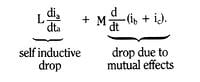
 But, in a balanced network, we must have 

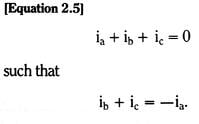
For the inductive voltage drop in the (a) phase, we then have

 We term the equivalent inductance, L-M, the positive sequence self-inductance.  Similar developments follow for capacitive and resistive coupling.

A solution for the (a) phase voltages (voltages to neutral) and currents in the resultant equivalent single-phase network (the positive sequence network) is then, in effect, a solution for the entire balanced three-phase network.  It is important to note that this technique is only applicable to completely balanced circuits, ones for which Equation 2.5, and a similar one for voltage, are true.

If there is an imbalance in the network, such as a fault in one of the phases, then the circuit voltages and currents will also no longer be balanced.  They will no longer be composed of just positive sequence components.

The easiest way to analyze the situation of a normally balanced three-phase circuit with a localized unbalanced section is to separate the total circuit into a balanced portion, usually almost the entire circuit, and an unbalanced portion, usually just the fault current path.  This method is commonly called the method of Symmetrical components.  The balanced portion is represented by three single-phase sequence networks.  The voltages and currents in the sequence networks are the normal mode voltages and currents of the balanced portion of the entire three-phase network.

The normal mode voltages and currents of an electrical network are those voltages and currents which match the normal, or natural, response of the network.  A balanced three-phase network has three normal modes; while a balanced two-phase network has only two normal modes.  A balanced six-phase network has six normal modes, and so on.  Normal modes of a network are distinctive in that they can be excited, and sustained, independent of one another.

We have already discussed one normal mode of symmetrical three-phase network, the positive sequence.  A second normal mode for a balanced three-phase network can be excited, if we simply reverse the phase order of the system drive voltages.  That is, instead of phases (a), (b) and (c), having the t=0 phase order, 0^o, -120^o and -240^o, we interchange the phasing of (b) and (c) so that the t=0 phase order for (a), (b) and (c) is 0^o, -240^o and -120^o.  This phase rotation, which appears in time as (a), (c), (b), is called the negative sequence phase rotation.  It is the same phase rotation that would occur if we mechanically drove all the generators in the three-phase network backwards, instead of their normal direction.

The positive and negative sequence phase rotations are shown in vector form in a complex plane in Figure 2.10. 

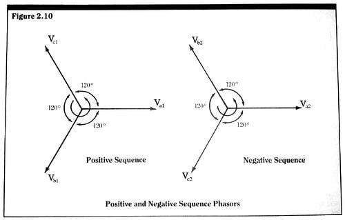
These vectors represent a snapshot of sequence voltages or currents at any one particular time.  The actual or real values of the sequence voltages or currents are the projections of the lengths of these vectors onto the horizontal real axis.  As time advances, these sets of sequence vectors rotate in a counter-clockwise direction in the complex plane at an angular frequency of 2πf.  This rotation can be seen quite clearly by studying the properties of the individual sequence vectors in the complex plane, which, for a sequence voltage, are of the form

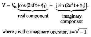
  The magnitude of this complex vector at all times is V_m, but, at any one particular time, V has different real and imaginary parts.  These real and imaginary parts are the components of the dimensional vector in the complex plane.  As time advances, the entire vector rotates in the counter-clockwise direction – that is, the arguments of the trigonometric functions advance – with angular frequency, 2πf.  The snapshot of the complex vectors at any one particular time is called a phasor diagram.  And the individual vectors in the diagram are termed phasors.  Note that each set of sequence phasors contains three equal magnitude (balanced) phasors.  The sequence components in each phase are always equal in magnitude.  Their only difference is their relative phasing.

The third normal mode for a balanced three-phase electrical network is one which is excited by having all drive generators, in all three phases, in phase.  This mode, or sequence, is called the zero sequence.  Zero sequence currents in phases (a), (b) and (c) are equal in magnitude (balanced) and in phase.  By Kirchoff’s current law, the total zero sequence current (three times the value in any one phase) must then return by some other path than the phase (a), (b) and (c) conductors.  For zero sequence currents to exist, there must be a fourth conductor (neutral or ground) return path.  Therefore, zero sequence currents cannot flow in a pure “delta system,” one with only three wires.

Zero sequence currents are often called unbalanced currents.  In the sense that they are the leftover currents after the positive and negative sequence balanced currents have been accounted for, the statement is true.  But it should be recognized that zero sequence currents are also balanced in the sense that equal amounts (one third of the total) of zero sequence current flow in each phase of a three-phase system.  A phasor diagram for zero sequence phasors is given in Figure 2.11.  It is particularly simple since all three phasors are the same, equal in magnitude and in phase.

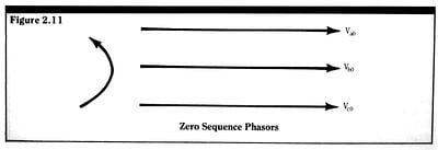
 The actual phase voltage or current can now be formed from its sequence or symmetrical components.  For example, since we have arbitrarily chosen phase (a) as the reference phase, the components of the (a) phase voltage add up algebraically.  That is,

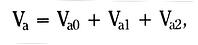
where V_a0, V_a1, and V_a2 are the zero, positive and negative sequence components of V_a, respectively.  Phase voltages, V_b and V_c, are also composed of their respective components

V_b = V_b0 + V_b1 + V_b2

and

V_c = V_c0 + V_c1 + V_c2

However, we must treat these additions as vector additions since the components, V_b1, V_b2, V_c1, and V_c2, have both real and imaginary parts.

The standard method of symmetrical components uses the (a) phase symmetrical components as the reference phase sequence components throughout, by defining a pure rotation operator as

A = cos 120^o + j sin 120^o.

When this operator is multiplied with a complex vector, it rotates the vector 120^o in the counter-clockwise direction.  Rotation by -120^o, which is the same as a +240^o rotation, is accomplished by a double +120^o rotation- that is, multiplication by a².  Thus we can form

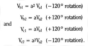
 We then have, in matrix form,

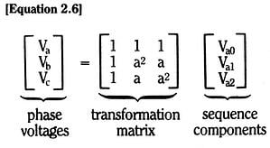
 By simple matrix inversion, we can also form

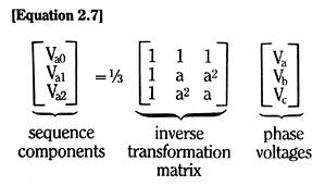
which is the definition of the (a) phase sequence components in terms of the actual phase quantities.  A similar set of equations can be developed for the relationships between the phase and the sequence currents.

The positive, negative and zero sequence modes are not the only set of normal modes that can be devised for a symmetrical three-phase electrical network.  However, they are the set most commonly used by electrical engineers and, as such, we will not consider any others.  In the development given here, our objective is to demonstrate, through the use of symmetrical components that faults in three-phase networks can be simplified and ultimately reduced to single-phase faulted networks.

As stated previously, in an unfaulted, completely balanced three-phase network, only positive sequence voltages and currents are excited.  Negative and zero sequence voltages and currents are not excited, and hence do not appear.  An unbalanced fault, however, will upset the circuit three-phase symmetry and potentially excite negative and zero sequence voltages and currents.  The degree of excitation is dependent on the type and position of the fault and the type of the three-phase circuit.  Just as in single-phase networks, we can use Thevenin equivalent networks to represent the sequence network portions of a balanced source network and a balanced load network.  And, just as in single-phase networks, we can combine the source and load portions of each sequence network, and arrive at a total Thevenin equivalent network, similar to the single-phase network in Figure 2.4.  This total sequence Thevenin equivalent network is shown in Figure 2.12.

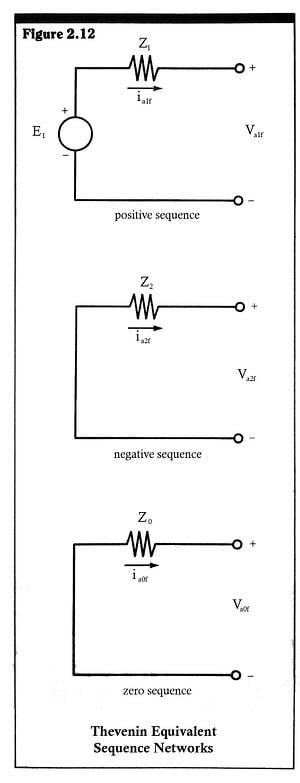
The positive sequence Thevenin network has an equivalent voltage source, E₁, and equivalent impedance, Z₁.  But the Thevenin networks for the negative and zero sequence networks have only internal equivalent impedances, Z₂ and X₀, respectively.  This is due to the fact that the negative and zero sequences have no steady-state excitation.

The terminals of the sequence Thevenin networks are called the fault terminals.  The voltages across these terminals are the sequence voltages at the point of the fault in the actual three-phase network.  And the sequence currents through these terminals are the sequence currents which flow through the fault path.

Consider now an example of an unbalanced fault.  Assume phase (a) is shunted to neutral through a fault resistance, R_f, as shown in Figure 2.13. 

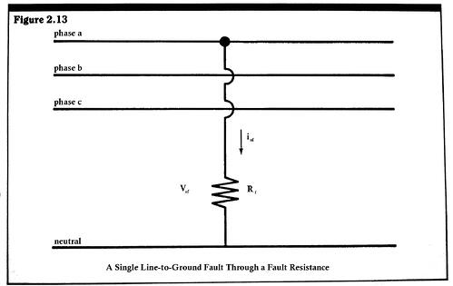
Since (b) and (c) phases are not involved in the fault, we have equations similar to Equation 2.6, thus,

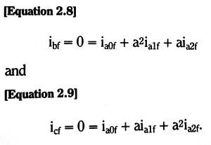
 If we subtract these two equations, we obtain

(a^2-a) i_alf = (a^2-a) i_a2f

which can be satisfied only if the positive and negative sequence components of the (a) phase current are equal.  Substituting this fact back into either Equation 2.8 or Equation 2.9, we see that we must also have

I_a0f = i_alf = i_a2f

This relationship is satisfied if all the sequence networks of Figure 2.12 are connected in series.  Also, at the fault point in the (a) phase, we must have

V_af = i_af R_f

or

V_a0f + V_alf + V_a2f = (i_a0f + i_alf + i_a2f) R_f = 3 R_f i_a0f.

Thus, the external load on the series connection of the three sequence networks is seen to be an equivalent fault resistance of value 3R_f.

The total sequence network connection is shown in Figure 2.14a. 

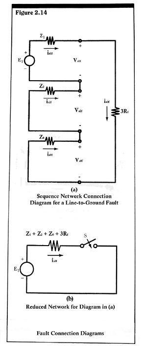
We can simplify the circuit of Figure 2.14a by combining all the impedances in series, to form one total impedance Z,

Z= Z₁ + Z₂ + Z₀ + 3R_f

And by redrawing, to obtain the equivalent form shown in Figure 2.14b. We have added a switch to illustrate that the fault is initiated at a particular time, t.

 Although this final form of the fault circuit is now in exactly the same form as the single-phase circuit of Figure 2.4, and can be solved in exactly the same manner as the single-phase circuit, the resulting solution is not the end product we seek.  The transient or steady-state current, solved for in the circuits of Figure 2.14a and Figure 2.14b, is the zero sequence component of the fault current.  The total (a) phase fault current is given by

I_af = 3i_a0f

This total fault current is then distributed throughout the (a) phase network in both the source and load portions of the total network.  Of course, this division of the total fault current among the source and load network occurs in single-phase circuits as well.

All types of faults in three-phase networks can be solved in a manner similar to that of the previous example.  The fault boundary conditions are expressed in terms of the sequence components, and the sequence Thevenin networks are connected to satisfy these boundary conditions.  The actual phase currents are then formed from the sequence currents, using an equation similar to Equation 2.6.

Before an electrical circuit interruption process is initiated – that is, when the contacts of an interrupting device start to open or the injection of mobile carriers into a semiconductor switch is restricted – the interrupting device must first make a trip/no-trip decision.  The period of time between the initiation of an overcurrent condition within a circuit and the initiation of interruptive action by the circuit protection device is termed the detection period.  The different types of protection devices detect overcurrents in different ways.  Thus, they can have different detection periods for the same overcurrent conditions. 

The detection mechanism in a fuse is the melting and the vaporization of a fusible link.  In a thermal breaker, dissimilar metals, bonded together along a single surface, expand differently under the direct or indirect resistive heating of the overcurrent.  This forces a lateral mechanical movement, perpendicular to the bonded surface, which releases a latched contact separation mechanism.  In some types of thermal breakers, the contact mechanism can be formed using the bi-metal material itself.  In these devices, the bi-metal arms/contacts snap open when they absorb sufficient energy from the circuit overcurrent.  Another form of thermal breaker utilizes the longitudinal expansion of a hot wire, which carries the overcurrent, to release a contact latch.

The detection portion of a magnetic breaker is comprised of an electromagnet driven by the circuit current.  An overcurrent will develop, within the electromagnet, enough magnetic pull to trip a spring restrained latch which, as in the thermal breaker, allows the spring loaded contacts to separate.

A solid-state switch detects overcurrents electronically, in many cases by simply monitoring the voltage drop across a low value resistance which carries the circuit current. 

Obviously, the faster a protection device can detect an overcurrent, the shorter the detection period.  But, in the majority of cases, the fastest possible detection speed is not desirable.  The speed of detection must be controllable and inversely matched to the severity of the overcurrent.

Series-connected protection devices must be coordinated.  For a given level of overcurrent, the device nearest to, and upstream from, the cause of the overcurrent must have the fastest response.  Devices which are further upstream must have a delayed response, such that the minimum circuit removal principle is adhered to.  When we speak of response, we are referring to the total response time, or total clearing time, of the interruption device, from the time of the overcurrent initiation to the final current-zero at which interruption is completed.  Since it is far easier to engineer the extent of the detection period for a given level of overcurrent than it is to control the extent of the actual current interruption process, the total response time of any protection device is, by design, determined principally by the size of, and the time required to detect, the overcurrent state.

The interruption period is defined as the length of time between the start of interruptive action – for example, when the contacts start to part – and the final current-zero.  The sum of the detection period and the interruption period is then the total clearing time, or total trip time, of the protection device.  These different time periods are shown in figure 1.5.

In contrast to the detection period, the interruption period cannot be engineered to decrease the intensity of an overcurrent increases.  The interruption period is, however, almost always designed to be as short as possible, since during this period the protection device is absorbing energy, due to the overcurrent flowing through the voltage drop across the contacts (or terminals in the case of a solid-state device).  If protection devices, other than fuses, do not clear the overcurrents fast enough during this period, they can be destroyed due to their own power dissipation.  Of course, fuses by design are always destroyed when they interrupt a circuit.

In AC circuits, the interruption period will last to either the first forced current-zero or the first natural current-zero at which the switching medium (arc or solid-state material) can reach its non-conducting blocking state.  In DC circuits, the current-zero state is always a result of a forcing action by the interrupting device. 
There are additional time periods of interest during the current interruption process, such as contact travel time, arc restrike voltage transient time, thermal recovery time, and charge storage time (for solid state devices). 

The voltage and current in a complete electrical circuit obey Kirchhof’s voltage and current laws.  These laws simply stated are:  the rises and drops in voltage around any closed circuit (a circuit loop) must sum to zero; and the total current flow into any one junction (connection point) must also sum to zero.  If we wish to interrupt the current in a circuit, we must do so in accordance with these laws.

Although it sounds simple, interrupt the circuit, break the conduction path, or open the switch – it is not.  Forcing a conducting circuit to a steady-state condition of zero current is anything but simple.  Many times, the actual detailed physics of the process of current interruption is obscured by the seeming triviality of the switching action – such as simply flicking off a flashlight.  But consider what actually happens when a flashlight is turned off.

A steady-state direct current (DC) is flowing from the batteries to the bulb as the switch contacts begin to move.  At the last microscopic points of electrical contact, the current density becomes high enough that portions of the metallic surfaces actually melt due to resistive heating; and a liquid metal vapor plasma state continues the electrical conducting path as the contacts physically part.  As the contacts pull further apart to distances of several microns (one micron = 10^-6 meters), electrons from the contact into which the current is flowing, the cathode contact, are emitted into the intercontact space region due to thermal emission (they boil off) and field emission (they are ripped from the cathode metal by electrostatic attraction forces).

A portion of these electrons emitted from the cathode collide with air molecules within the contact gap and ionize the molecules. This frees still more electrons, which in turn ionize still more air molecules.  This self-perpetuating action is an electrical breakdown phenomenon commonly referred to as an arc.  It is the arc which enables the switch to open the circuit.  The arc forms just as the contacts part, and continues to conduct the circuit current as the contacts move further and further apart.

The voltage drop across the arc – which is proportional to the arc length and inversely proportional to the arc cross-sectional size – is in series with the voltages in the circuit loop which contains the switch.  The arc voltage grows as the arc is lengthened by the physical movement of the contacts, and the arc cross-section is diminished as the arc is cooled by contact with un-ionized air molecules.

The arc voltage in low voltage DC circuits grows at such a rate that it soon exceeds, or at least matches, the source voltage in the circuit (in a flashlight the initial arc voltage exceeds the battery voltage).  When this occurs, the circuit current is driven to zero in short order.  All circuits contain a small but finite inductance, so the current cannot be driven to zero instantaneously.  When the current does reach zero, no further arc ionization takes place, and the arc is cooled even more rapidly, since it has no energy input.  If it is cooled momentarily to such a state that it is no longer a conducting medium, then the interruption process is complete and the circuit has been opened.  It is important to remember that it is the arc that forces the current to zero.  The opening of the switch forms the arc, but it is the arc which enables the circuit to be interrupted.

A switch or circuit interruption device which is intended to open alternating current (AC) circuits has a somewhat easier chore than its DC counterpart.  In AC circuits, there is no need to force a current-zero condition.  Since the current alternates about zero already, there is a natural current-zero twice in each AC cycle.  Any arc which forms in an AC switching device does not have to be stretched and cooled to the extent that the arc voltage exceeds the magnitude of the circuit source voltage.   However, this can be done if one wishes to limit the magnitude of an overcurrent by driving it down to an unnatural current-zero.

AC currents can be interrupted at a natural current-zero, which is primarily determined by the circuit alone and practically unaffected by the presence of the interruption device.  Alternately, AC currents can be interrupted at forced current-zeros, which are imposed by the action of the interruption device.  Figure 1.3 illustrates these concepts of natural and forced current-zeros in an AC circuit.

All mechanical switches and mechanical circuit interrupting devices depend on the rapid cooling of the arc medium to open an electrical circuit.  Solid-state switches do not need an arc to break a circuit, since they supply their own conducting medium, the semiconductor material itself.  A semiconductor can conduct current only as long as mobile carriers (electrons and holes) are provided from supply or injection regions within the device.  If the injection of mobile carriers in a semiconductor switch is turned off, then the semiconductor material will revert to an insulating state and block the flow of current – that is, the semiconductor switch will turn off.

The allowable current density within a semiconductor switch is much lower than that which can safely flow in a metal contact/arc switch.  Thus, the cross-sectional size of a semiconductor switch, for equal rating devices, will always be larger than that of a mechanical switch.  Even with this disadvantage, the ease with which a semiconductor switch can be controlled, and the reliability of a device with no mechanically moving parts, portends a bright future for solid-state power switches and circuit breakers.

Overcurrents and protective devices are not new subjects.  Soon after Volta constructed his first electrochemical cell, or Faraday spun his first disk generator, someone else graciously supplied these inventors with their first short circuit loads.  Patents on mechanical circuit-breaking devices go back to the late 1800’s and the concept of a fuse goes all the way back to the first undersized wire that connected a generator to a load.

In a practical sense, we can say that no advance in electrical science can proceed without a corresponding advance in protection science.  An electric utility company would never connect a new generator, a new transformer, or a new electrical load to a circuit that cannot automatically open by means of a protective device.  Similarly, a design engineer should never design a new electronic power supply that does not automatically protect its solid-state power components in case of a shorted output.  Protection from overcurrent damage must be inherent to any new development in electrical apparatus.  Anything less leaves the apparatus or circuit susceptible to damage or total destruction within a relatively short time.  

The principles discussed in this brief are derived from Mechanical Products’ foundational publication, The Theory and Practice of Overcurrent Protection [1] . 

Examples of overcurrent protection devices are many:  fuses, electromechanical circuit breakers, and solid state power switches.  They are utilized in every conceivable electrical system where there is the possibility of overcurrent damage.  As a simple example, consider the typical industrial laboratory electrical system shown in Figure 1.1.  We show a one-line diagram of the radial distribution of electrical energy, starting from the utility distribution substation, going through the industrial plant, and ending in a small laboratory personal computer.  The system is said to be radial since all branch circuits, including the utility branch circuits, radiate from central tie points.  There is only a single feed line for each circuit.  There are other network type distribution systems for utilities, where some feed lines are paralleled.  But the radial system is the most common and the simplest to protect. [1]

Overcurrent protection is seen to be a series connection of cascading current-interrupting devices.  Starting from the load end, we have a dual-element or slow-blow fuse at the input of the power supply to the personal computer.  This fuse will open the 120 volt circuit for any large fault within the computer.  The large inrush current that occurs for a very short time when the computer is first turned on is masked by the slow element within the fuse.  Very large fault currents are detected and cleared by the fast element within the fuse.  

Protection against excess load at the plug strip, is provided by the thermal circuit breaker within the plug strip.  The thermal circuit breaker depends on differential expansion of dissimilar metals, which forces the mechanical opening of electrical contacts.  

The 120 volt single-phase branch circuit, within the laboratory which supplies the plug strip, has its own branch breaker in the laboratory’s main breaker box or panel board.  This branch breaker is a combination thermal and magnetic or thermal-mag breaker.  It has a bi-metallic element which, when heated by an overcurrent, will trip the device.  It also has a magnetic-assist winding which, by a solenoid type effect, speeds the response under heavy fault currents.

All of the branch circuits on a given phase of the laboratory’s 3-phase system join within the main breaker box and pass through the main circuit breaker of that phase, which is also a thermal magnetic unit.  This main breaker is purely for back up protection.  If, for any reason, a branch circuit breaker fails to interrupt overcurrents on that particular phase within the laboratory wiring, the main breaker will open a short time after the branch breaker should have opened.

Back-up is an important function in overload protection.  In a purely radial system, such as the laboratory system in Figure 1.1, we can easily see the cascade action in which each overcurrent protection device backs up the devices downstream from it.  If the computer power supply fuse fails to function properly, then the plug strip thermal breaker will respond, after a certain coordination delay.  If it should also fail, then the branch breaker should back them both up, again after a certain coordination delay.  This coordination delay is needed by the back-up device to give the primary protection device – the device which is electrically closest to the overload or fault – a chance to respond first.  The coordination delay is the principal means by which a back-up system is selective in its protection. [1]

Selectivity is the property of a protection system by which only the minimum amount of system functions are disconnected in order to alleviate an overcurrent situation.  A power delivery system which is selectively protected will be far more reliable than one which is not. [1]

For example, in the laboratory system of Figure 1.1, a short within the computer power cord should be attended to only by the thermal breaker in the plug strip.  All other loads on the branch circuit, as well as the remaining loads within the laboratory, should continue to be served.  Even if the breaker within the plug strip fails to respond to the fault within the computer power cord, and the branch breaker in the main breaker box, is forced into interruptive action, only that particular branch circuit is de-energized.  Loads on the other branch circuits within the laboratory still continue to be served.  In order for a fault within the computer power cord to cause a total blackout within the laboratory, two series-connected breakers would have to fail simultaneously – the probability of which is extremely small.

The ability of a particular overcurrent protection device to interrupt a given level of overcurrent depends on the device sensitivity.  In general, all overcurrent protection devices, no matter the type or principles of operation, respond faster when the levels of overcurrent are higher. [1]

Coordination of overcurrent protection requires that application engineers have detailed knowledge of the total range of response for particular protection devices.  This information is contained in the “trip time vs. current curves,” commonly referred to as the trip curves.  A trip time-current curve displays the range of, and the times of response for, the currents for which the device will interrupt current flow at a given level of circuit voltage.  For example, the time current curves for the protection devices in our laboratory example are shown superimposed in Figure 1.2.

The rated current for a device is the highest steady-state current level at which the device will not trip for a given ambient temperature.  The steady-state trip current is referred to as the ultimate trip current.  The ratings for the dual-element fuse in the computer power supply, the plug strip thermal breaker, the branch circuit thermal-magnetic breaker and the main circuit thermal-magnetic breaker are 2, 15, 20, and 100 amps, respectively.  Note that, except for the fuse curve, each time-current curve is shown as a shaded area, representing the range of response for each device.  Manufacturing tolerances and material property inconsistencies are responsible for these banded sets of responses.  Trip time-current information for small fuses is usually represented in a single-value average melting time curve.

Even with a finite width to the time-current curves, we can easily see the selectivity/coordination between the different protection devices.  For any given steady-state level of overcurrent, we read up the trip time-current plot, at that level of current, to determine the order of response.

Consider the following three examples for the laboratory wiring, plug strip, and computer system.  

Example 1: Component failure within the computer power supply:  Assume that a power component within the computer power supply has failed – say two legs of the bridge power rectifier – and that the resulting fault current within the supply, limited by a surge resister, is 70 amps.

We see from the fuse trip curve that it should clear this level of current in approximately 20 milliseconds.  If the fuse fails to interrupt the current – or worse, if the fuse has been replaced with a permanent short circuit by a gambling repairperson – the thermal breaker in the plug strip should open the circuit within 0.6 to 3.5 seconds.  The branch thermal-magnetic breaker will open the entire branch circuit within 3.5 to 7.0 seconds, should the plug strip thermal breaker also fail to respond. [1]

Note that no back-up is provided for this particular fault after the branch circuit breaker.  The main laboratory 100 amp thermal-magnetic unit would respond only if the other loads within the entire laboratory totaled greater than 30 amps at the time of the 70 amp power supply fault.

Example 2:  Plug strip overload:  Assume that the computer operator has spilled a drink, and to dry up the mess plugs two 1500 watt hair dryers into the plug strip.  The operator then flips them both on simultaneously, drawing a total plug strip load current of approximately 30 amps.

From the thermal breaker trip curve, we see that the plug strip unit should clear this overload within 5 to 30 seconds.  Note the similarity between the trip curves of the plug strip thermal unit and the branch circuit thermal-magnetic unit in the region of 100 amps and below.  This is because, for these levels of currents, the thermal portion of the detection mechanism within the thermal-magnetic branch breaker is dominant. 

Example 3:  Short circuit within the computer power cord:  Assume a frayed line cord finally shorts during some mechanical movement.  Assume also that there is enough resistance within the circuit, plug strip, and line cord system to limit the resulting fault current to 300 amps.  This level of current is 2000% (20 times) of the rated current of the plug strip thermal breaker, and is beyond the normal range of published trip time specifications for thermal breakers (100% to 1000% of rated current).  Thus the exact trip time range of the thermal unit is indeterminate.

At high levels of fault current, greater than 150 amps in this case, we can see the inherent speed advantage of magnetic detection of overcurrents.  This is evidenced by the fact that the response curve for the thermal-magnetic branch circuit breaker knees downward sharply at current levels between 150 and 200 amps.  At these and higher currents, the magnetic detection mechanism within the thermal-magnetic unit is dominant.  The response curve for the unit crosses over the plug strip thermal breaker response curve (assuming that it extends past its 1000% limit), and coordination between the two interrupters is lost.  The range of response for the thermal-magnetic breaker at 300 amps is 8 to 185 milliseconds.  Should both the plug strip breaker and the branch circuit breaker fail to operate, the main laboratory breaker should clear the fault within 11 to 40 seconds. [1]

 References [1] P. J. McCleer, The Theory and Practice of Overcurrent Protection. Chelsea, MI: BookCrafters, Inc., 1987. ISBN: 0-9618814-0-2. 

If you’re looking to source thermal circuit protection, look no further.  MP’s 40+ years of excellent reputation in thermal breakers is unmatched in the industry, and offers protection from ½ to 70 amperes, in Push to Reset and Switchable versions.  All are ROHS compliant with a broad range of Worldwide accepted agency approvals.  Standard variations or custom requirements are offered for a variety of applications in the Construction, Marine, Medical, RV, Power Generation, Appliance, Floor Care and specialty applications.  Competitive pricing with volume discounts are available for these high quality thermal circuit protectors.  So don’t settle for just any circuit breaker.  Ask for Mechanical Products, a market leader in thermal circuit protection.   Contact Mechanical Products at helpme@mechprod.com.