Our concern, here, is overcurrent protection, so we will restrict our attention to one particular location within a circuit, the location, or potential location of an interruptive device. We arbitrarily divide the total circuit into two sections: a delivery, or source, electrical network; and a load electrical network (Figure 2.1). These two networks are connected by two current paths, one of which contains the interruptive device.
If both the source network and the load network are linear – a common approximation which is entirely adequate for fault transient calculations – we can, by Thevenin’s theorem (2.1), replace each network by an equivalent source voltage, E, and equivalent network impedance, Z. The equivalent source voltage for each network is the voltage which would be measured at the network terminals under open circuit (no load) conditions. The equivalent network impedance is a mathematical description of the combination of resistances, capacitances and inductances that would be measured at the open circuit network terminals. The equivalent Thevenin networks for the source and load networks are shown in Figure 2.2. 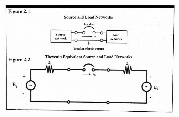

The voltages, E1 and E2, represent the equivalent voltage sources for the source network and load network, respectively. The source network voltage, E1, represents all the combined voltage generators within the source network. For Example, if the source network is a feed from an electric utility network, then E1 represents the thousands of generators connected to the utility network, as measured under open circuit conditions at the source network terminals. But, if the source network is an equivalent for an aircraft 28 volt DC electrical network, E1 represents the rectified alternator output, as measured under open circuit conditions at the source network terminals.
The load network voltage source, E2, represents all of the combined voltage generators within the load network. Many times there are no voltage sources within the load network, so E2 is zero. But, if the load network contains a source, such as the electromotive force (emf) in the windings of a motor, E2 represents the combined total load network voltage, as measured under open circuit conditions at the load network terminals.
The network impedance elements, Z1 and Z2, represent equivalent impedances for the source and load networks, respectively. The impedance of the interrupting device itself can be arbitrarily lumped in with either the source or the load impedance, Z1 or Z2.
If the source network is an equivalent for a 120 volt wall outlet, then Z1 represents the combined impedances of the thousands of transmission lines, transformers and generator windings which make up the feeding utility network; and the impedances of the local wiring network which connects the outlet. If the source network is an equivalent for an aircraft network then Z1 represents only the interior wiring within the airplane and the internal impedances of the alternator, as measured at the network terminals.
In a practical sense, the dominant contributors to Z1 in a largesource network are only those network elements which are physically close to the source network terminals. In a large factory electrical network, the dominant terms in Z1 are the impedances of the wires which connect the source network terminals to the nearest substation transformer, and the impedance of the nearest substation transformer windings. In smaller networks, such as an automotive network, all impedance terms must be accounted for in Z1, since they all make significant contributions.
For example, in the simple automotive network shown in Figure 2.3, the internal resistance of the twelve volt automobile battery limits the initial short circuit current at the battery’s terminals to 2000 amps. But, if the short is at the terminals of the starter motor, the initial short circuit current would be only 1500 amps. Clearly the additional resistance of the wiring from the battery to the starter motor is responsible for this reduction in potential short circuit current. The additional resistance is comparable in value to the internal resistance of the battery. 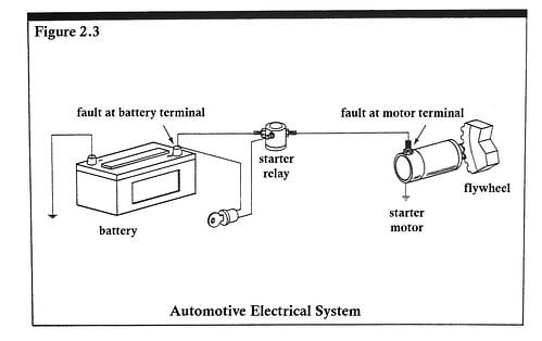
Contrast this case, where the impedances of all network elements are important, to the example of a large factory system. In a large industrial system, it would make negligible difference to an individual user at a particular work station if one or even ten generators were added to the electric utility system which feeds the factory substation. The value of a work station’s perceived system impedance, Z1, would not change to any significant degree.
The equivalent load impedance, Z2, represents the load network passive elements, as measured from the load network terminals. Just as in the case of Z1, only dominant elements need be accounted for when computing system currents.
The equivalent network of Figure 2.2 can be simplified even further, if we make the following substitutions: 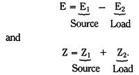
We then obtain the simplified circuit of Figure 2.4. Observe that a solution of the electrical network equations for this circuit will give us a solution for the breaker current, ib. Also observe that it does not matter whether this circuit represents the steady-state operation of our system, or the operation during a system transient due to some sudden change in the system network. 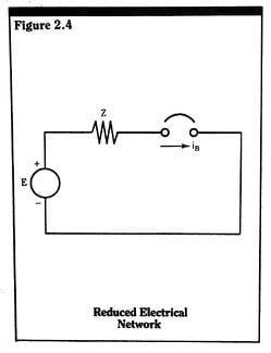
We will use the equivalent network of Figure 2.4 to represent the transient operation of an electrical circuit, and from it derive the transient behavior of the breaker current, iB. Before the transient, assumed to start at time t=0, the breaker may be passing some value of pre-transient current, iB0. We can use this value as a boundary condition in our transient solution. We can be assured, however, that iB0 is within the rating of the breaker and/or circuit, since, by definition, we are asserting that only under transient conditions will any rated value of circuit current or voltage be exceeded.
We now give an example of circuit reduction to the form of Figure 2.4. If we choose a thermal breaker within a plug strip as our study breaker, then the reduced networks – which are equivalent to the single-phase feed from the utility through the plant and laboratory wiring and the power supply load – can be represented as shown in Figure 2.5. 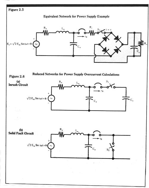
The source side inductance LW, and the resistance RW, represent the inductance and resistance of the wiring from the utility substation transformer to the plug strip, and the inductance and resistance of the utility substation transformer itself. We will also include with LW and RW any inductance and resistance within the breaker mechanism itself. The source side capacitance, CW, represents a lumped approximation for the distributed capacitance of the supply wiring to ground, and the transformer windings to ground. The source voltage, ES, is a 60 Hz sinusoidal voltage with RMS (root mean square) magnitude, Em = 120 V, and a phase angle, o. The power supply load is represented by a wiring resistance, Rc, a series connected on/off switch, S1, a full wave diode rectifier, and a parallel R0, C0 load.
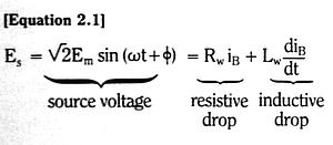
A transient overcurrent could occur any number of ways in this circuit. Figure 2.6 illustrates two of the most common. A start-up transient is shown in Figure 2.6a. Here, the on/off switch, S1, is closed at t = 0, and the load capacitor, C0, is assumed to be uncharged before t = 0. Once C0 is charged, the line current through the breaker settles down to its rated value or below, dependent on the equivalent load resister, R0. The circuit in Figure 2.6a neglects the rectifying action of the diode bridge and the load resistor, R0, during the start-up transient. Analysis of this particular circuit would be a conservative method of calculating the start-up transient behavior of iB. Note that the circuit in Figure 2.6a is of the same form as our general transient equivalent circuit, as given in Figure 2.4.
The second type of transient overcurrent which we will consider for the plug strip and computer power supply circuit is the worst case transient – a permanent short circuit at the input to the computer line cord. The equivalent circuit for this condition is shown in Figure 2.6b. Here, the computer load does not enter into the transient calculation, since it is completely shorted out by the equivalent shorting switch, S2, which closes at t = 0. Also shorted for all practical purposes, and thus irrelevant to the analysis, is the source shunt capacitance, CW. Note again that the resultant circuit is of the same topology as the general transient circuit of Figure 2.4.
Prior to the short, any prefault line current flowing through the breaker in Figure 2.6b is treated as a t = 0 boundary condition for iB. The solution for the breaker current is the complete solution, both transient and steady-state, to the differential equation which describes Kirchoff’s voltage law around the Es-LW-Rw loop. Namely:
 Where w=2
![]() f is the system drive radian frequency, with f=60Hz. The total solution to Equation 2.1, from the elementary theory of differential equations, is
f is the system drive radian frequency, with f=60Hz. The total solution to Equation 2.1, from the elementary theory of differential equations, is 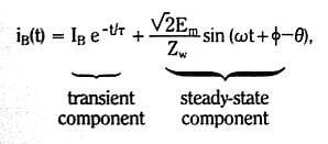
Where Ƭ is the source inductive time constant, LW/RW; Zw is the inductive impedance at the driving frequency f, ![]()
Xwis the source network inductive reactance, XW=wLW; and the 0 is the angle by which the steady-state short circuit current lags the drive voltage Es, ![]()
The constant IB must be determined from the boundary condition for iB. Since iB=iBo at t = 0, we have 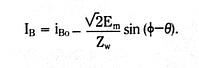
If we define the symmetrical RMS short circuit current magnitude as 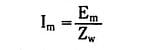
Then, for the complete time variation of the short circuit breaker current, we have
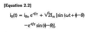
In nearly all cases, the magnitude of the steady state short circuit current is much greater than the pre-fault current (which is within the rated value of the circuit). So we can easily neglect the first term in Equation 2.2. We then have
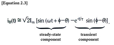 Equation 2.3 is plotted in Figures 2.7a through 2.7e, normalized to
 ![]() , as a function of the product ft. Note that
, as a function of the product ft. Note that 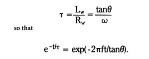
In Figures 2.7a through 2.7e, the system impedance angle, 0, is specified, varying from 5o to 85o. Since the fault would be a random event, the switching angle, φ, could be any value over a 360o range. We show individual iB curves for discrete values of φ, varying from φ=180o to +180o in 30o increments. These sets of curves for the different values of φ then form waveform envelopes, in which any time variation of iB will lie.
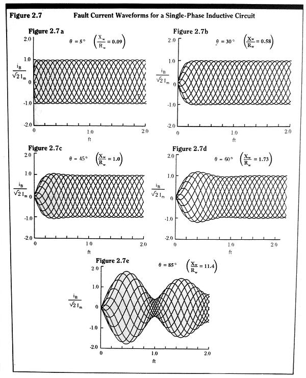
Of interest, in the results shown in Figures 2.7a through 2.7e, is the transient bulge in the iB envelopes for circuits with largely inductive (0>45o) system impedances. The more inductive the circuit, the greater the bulge. This effect is due to the inertial property of the magnetic flux within the system inductance. Mathematically, it is evidenced in the second term in Equation 2.3. This term is referred to as the DC offset in the line current. It decays exponentially, with a time constant equal to LW/RW, and has a maximum initial value when the angular difference between the switching angle, φ, and the system impedance angle, 0, is +/- 90o.
The principal consequence of the DC offset is the potential for fault current levels through the breaker to be almost twice the level of the peak steady-state or sustained fault current level. The phenomenon is seen more clearly in Figure 2.8, where four cycles of an almost fully offset current waveform are shown. As can be seen, the line current at one half cycle into the fault is approximately 1.75 times the peak fault current after the offset transient has died down.
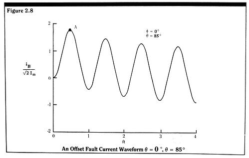
In general, low voltage (240/120V) circuits in industrial and household installations have enough wiring between the circuit and the utility system, so that the system X over R ratio is less than unity (i.e. 0<45o). Thus, these circuits do not experience offset fault currents. Fault currents, such as those shown in the waveforms of Figure 2.7 and 2.8, must pass non-destructively through the breaker mechanism. The peak potential current (point A in Figure 2.8) in a fault waveform is termed the peak value of the prospective fault current. This current value must be less than, or equal to, the interruptive capacity of the breaker (the maximum amount of current a breaker can interrupt, while still able to function if reset).
If the breaker or the fuse is a “current limiting” type device, then the peak prospective fault current is the peak fault current that would flow if the limiting device were not present. The actual peak fault current would be less than the peak prospective fault current, and would depend on the amount of additional circuit impedance that is inserted by an interruptive device mechanism. Usually, this additional impedance is in the form of an elongated arc, such as that in a fuse or cooled arc chamber. Thus, the waveforms of Figures 2.7 and 2.8 do not apply to fault currents which are limited by current limiting type breakers. They apply only to the perspective fault currents for these types of breakers.
If the generalized circuit of Figure 2.4 represents a DC circuit wherein the source voltage is a simple DC voltage with magnitude E0, the solution for the transient breaker current, iB, is considerably simpler. For the loop voltage equation, we have 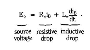
The solution for this equation, again from the theory of elementary differential equations, is 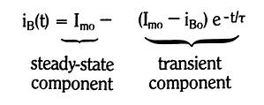
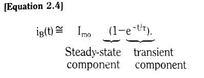
where, as before, iBo is the prefault (t=0) breaker current and Ƭ is the source system time constant, LW/RW. The steady state sustained fault current, Imo, is simply the pure resistive current, 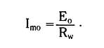
As in the single-phase AC case, the steady-fault current is generally much larger than the prefault current, iBo, so that we can approximate the transient fault current by
This waveform is shown in Figure 2.9, normalized to Imo.
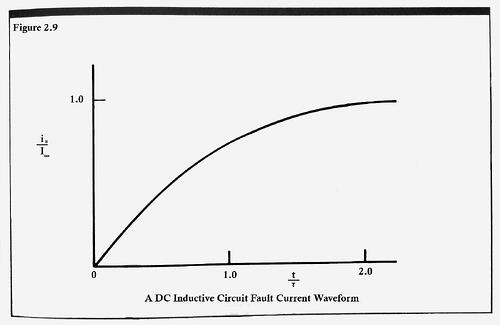
Note that in this DC case there are no switching angles or timing considerations. The fault current simply rises exponentially to its steady state value, governed by the system time constant Ƭ. The peak prospective fault current is the steady-state fault current, Imo, and there are no offset currents that add to this value. The complication, if there is any in a DC circuit, is that the fault current is truly a unipolar current with no natural current-zero. A DC breaker must then force a current-zero in order to interrupt the circuit.